NON-MONOTONIC REASONING FOR REQUIREMENTS

ENGINEERING

State Diagrams Driven by Plausible Logic

David Billington, Vladimir Estivill-Castro, Rene Hexel and Andrew Rock

School of ICT, Grifﬁth University, Nathan Campus, Nathan, 4111 Queensland, Australia

Keywords:

Automata and logic for system analysis and veriﬁcation, Petri nets, Requirements engineering.

Abstract:

We extend the state diagrams used for dynamic modelling in object-oriented analysis and design. We sug-

gest that the events which label the state transitions be replaced with plausible logic expressions. The result

is a very effective descriptive and declarative mechanism for specifying requirements that can be applied to

requirements engineering of robotic and embedded systems. The declarative model can automatically be trans-

lated and requirements are traceable to implementation and validation, minimising faults from the perspective

of software engineering. We compare our approach with Petri Nets and Behavior Trees using the well-known

example of the one-minute microwave oven.

1 INTRODUCTION

We extend state transition diagrams in that we al-

low transitions to be labelled by statements of a non-

monotonic logic, in particular Plausible Logic. We

show that this has several beneﬁts. First, it facilitates

requirements engineering. Namely, we show this ap-

proach can be more transparent, clear, and succinct

than other alternatives. Therefore, it enables better

capture of requirements and this leads to much more

effective system development. Furthermore, we show

that such diagrams can be directly, and automatically

translated into executable code, i.e. no introduction of

failures in the software development process.

Finite automata have a long history of mod-

elling dynamic systems and consequently have been

a strong inﬂuence in the modelling of the behaviour

of computer systems (Rumbaugh et al., 1991, Biblio-

graphical notes, p. 113-114). System analysis and de-

sign uses diagrams that represent behaviour of com-

ponents or classes. State diagrams (or state machines)

constitute the core behavior modeling tool of object-

oriented methodologies. In the early 90s state ma-

chines became the instrument of choice to model the

behaviour of all the objects of a class. The Object-

Modeling Methodology (OMT) of Rumbaugh et al.

(1991, chapter 5) established state diagrams as the pri-

mary dynamic model. The Shlaer-Mellor approach

established state models to capture the life cycle of

objects of a given class (Shlaer and Mellor, 1992).

Class diagrams capture the static information of all

objects of the same class (what they know, what they

store), but behaviour is essentially described in mod-

els using states and transitions. The prominence of

OMT and Shlaer-Mellor has permeated into the most

popular modelling language for object-orientation,

the Uniﬁed Modeling Language (UML). “A state di-

agram describes the behavior of a single class of ob-

jects” (Rumbaugh et al., 1991, p. 90). Although the

state diagrams for each class do not describe the in-

teractions and behaviour of several objects of diverse

classes in action (for this, UML has collaboration dia-

grams and sequence diagrams), they constitute a cen-

tral modelling tool for software engineering.

Although UML and its variants have different lev-

els of formality, in the sense of having a very clear

syntax and semantics, they aim for the highest for-

mality possible. This is because their aim is to re-

move ambiguity and be the communication vehicle

between requesters, stakeholders, designers, imple-

mentors, testers, and users of a software system.

Thus, they offer constraints very similar to the for-

mal ﬁnite state machine models. For example, in a

deterministic ﬁnite state machine, no two transitions

out of the same state can be labelled with the same

symbol. This is because formally, a deterministic ﬁ-

nite state machine consists of a ﬁnite set of states, an

input language (for events), and a transition function.

The transition function indicates what the new state

will be, given an input and the current state. Other

Billington D., Estivill-Castro V., Hexel R. and Rock A. (2010).

NON-MONOTONIC REASONING FOR REQUIREMENTS ENGINEERING - State Diagrams Driven by Plausible Logic.

In Proceedings of the Fifth International Conference on Evaluation of Novel Approaches to Software Engineering, pages 68-77

DOI: 10.5220/0002998300680077

 SciTePress

Table 1: The Transition Function as a Table.

. . .

adornments include signalling some states as initial

and some as ﬁnal. However, a fundamental aspect of

ﬁnite state machines is that the transition function is

just that, a function (mathematically, a function pro-

vides only one value of the codomain for each value

in the domain).

Granted that the model can be extended to a non-

deterministic machine, where given an input and a

state, a set of possible states is the outcome of the

transition. In this case, the semantics of the behaviour

has several interpretations. For example, in the the-

ory of computation, the so-called power set construc-

tion shows that non-deterministic and deterministic

ﬁnite state machines are equivalent. However, other

semantics are possible, such as multi-threaded be-

haviour. Therefore, as a modelling instrument in soft-

ware engineering, it is typically expected that the con-

ditions emanating from a state are mutually exclu-

sive and exhaustive. “All the transitions leaving a

state must correspond to different events” (Rumbaugh

et al., 1991, p. 89). Namely, if the symbol c

is a

Boolean expression representing the guard of the tran-

sition, then

i=1

= true (the exhaustive condition),

and c

∧c

= false, ∀ i 6= j (the exclusivity condition).

In fact, Shlaer-Mellor also suggest the analysis should

make use of the State Transition Table (STT) (Shlaer

and Mellor, 1992). Table 1 is the tabular represen-

tation of the transition function “to prevent one from

making inconsistent statements” (Shlaer and Mellor,

1992, p. 52) and they provide an illustration where

two transitions out of the same state and labelled by

the same event are corrected using the table.

Recently, the software engineering community

has been pushing for Requirements Engineering

(RE) (Hull et al., 2005), concerned with identifying

and communicating the objectives of a software sys-

tem, and the context in which it will be used (Nu-

seibeh and Easterbrook, 2000). Hence, RE identiﬁes

and elicits the needs of users, customers, and other

stakeholders in the domain of a software system. RE

demands a careful systematic approach. Signiﬁcant

effort is to be placed on rigorous analysis and docu-

mented speciﬁcation, especially for security or safety

critical systems. RE is important because a require-

ment not captured early may result in a very large ef-

fort to re-engineer a deployed system.

2 NON-MONOTONIC LOGIC IN

STATE DIAGRAMS

An ambition of both artiﬁcial intelligence (AI) and

software engineering is to be able to only specify

what we want, without having to detail how to achieve

this. The motivation for our approach has a simi-

lar origin. We aim at producing a vehicle of com-

munication that would enable the speciﬁcation of be-

haviour without the need for imperative programming

tools. Therefore, we want to use a declarative formal-

ism (a similar ambition has lead to the introduction

of logic programming and functional programming).

Non-monotonic logic is regarded as quite compati-

ble with the way humans reason and express the con-

ditions and circumstances that lead to outcomes, as

well as a way to express the reﬁnements and even ex-

ceptions that polish a deﬁnition for a given concept.

In fact, non-monotonic reasoning is regarded as one

of the approaches to emulate common-sense reason-

ing (Russell and Norvig, 2002). We illustrate that the

addition of this declarative capability to state transi-

tion diagrams for capturing requirements is beneﬁcial

because the models obtained are much simpler (a fact

necessary to ensure that the natural language descrip-

tion has indeed been captured). This way, we only

need to specify the what and can have all of the how

within an embedded system generated automatically.

With our approach, modelling with state-diagrams

is sufﬁcient to develop and code behaviours. The se-

mantics of a state is that it is lasting in time, while a

transition is assumed to be instantaneous. The state-

diagram correspondsclosely to the formalism of ﬁnite

state machines (deﬁned by a set S of states, a transi-

tion function t : S× ϒ → S, where ϒ denotes a possi-

ble alphabet of input symbols). In our case, we can

specify the behaviour by the table that speciﬁes the

transition function t (Table 1).

We still use the notion of an initial state s

, be-

cause, in our infrastructure that implements these

ideas (Billington et al., 2009), in some external-state

transition, behaviours must be able to reset them-

selves to the initial state. A ﬁnal state is not required,

but behaviours should be able to indicate completion

of a task to other modules. Now, current practice

for modelling with ﬁnite state machines assumes that

transitions are labelled by events. In both the Shlaer-

Mellor approach and OMT (Rumbaugh et al., 1991),

transitions are labelled by events only. For exam-

ple, in Fig. 1, a transition is labelled by the event

ball visible

(e.g. a sensor has detected a ball). A

slight extension is to allow labels to be a decidable

Boolean condition (or expression) in a logic with val-

ues

true

false

(that is, it will always be possi-

NON-MONOTONIC REASONING FOR REQUIREMENTS ENGINEERING - State Diagrams Driven by Plausible Logic

Figure 1: Simple Finite State Diagram.

ble to ﬁnd the value of the condition guarding the

transition). This easily captures the earlier model be-

cause rather than labelling by event e, we label by

the Boolean expression e has occured. Our exten-

sion to behaviour modelling extends this further with

the transition labels being any sentence in the non-

monotonic logic. Replacing the guarding conditions

with statements in the non-monotonic logic incorpo-

rates reasoning into the reactive

nature of state ma-

chines. Since our logics model reasoning (and be-

liefs like “in this frame vision believes there is no

ball”), they are better suited to model these transitions

(they may even fuse contradicting beliefs reported by

many sensors and modules in a deterministic way),

and gracefully handle situations with incomplete (or

superﬂuous) information without increasing the cog-

nitive load of the behaviour designer.

The designer can separate the logic model from

the state-transition model. Moreover, the designer

would not be required to ensure the exhaustive nature

of the transitions leading out from a state; as priorities

can indicate a default transition if conditions guarding

other transitions cannot be decided.

“State diagrams have often been criticized be-

cause they allegedly lack expressive power and are

impractical for large problems” (Rumbaugh et al.,

1991, p. 95). However, several techniques such as

nesting state diagrams, state generalisation, and event

generalisation were used in OMT to resolve this issue.

We have shown elsewhere (Billington et al., 2010)

(1) how the technique of nested state diagrams (e.g.

team automata (ter Beek et al., 2003; Ellis, 1997)

handle complexity, and (2) that there is an equiv-

alence between Behavior Trees and state machines,

mitigating the problem of expressive power of state

diagrams for larger systems. In fact our approach fol-

lows the very successful modelling by ﬁnite state ma-

chines (Wagner et al., 2006) that has resulted in state-

WORKS, a product used for over decade in the engi-

neering of embedded systems software (Wagner and

Wolstenholme, 2003). In stateWORKS, transitions

are labelled by a small subset of propositional logic,

namely positive logic algebra (Wagner and Wolsten-

In the agent model reactive systems are seen as an al-

ternative to logic-based systems that perform planning and

reasoning (Wooldridge, 2002).

holme, 2003), which has no implication, and no nega-

tion (only OR and AND). Thus our use of a non-

monotonic logic is a signiﬁcant variation.

3 PLAUSIBLE LOGIC

Non-monotonic reasoning (Antoniou, 1997) is the ca-

pacity to make inferences from a database of be-

liefs and to correct those as new information arrives

that makes previous conclusions invalid. Although

several non-monotonic formalisms have been pro-

posed (Antoniou, 1997), The β algorithm for PL uses

the closed world assumption while the π algorithm

uses the open world assumption. the family of non-

monotonic logics called Defeasible Logics has the

advantage of being designed to be implementable.

The main members of this family, including Plausible

Logic (PL), are compared in (Billington, 2008), list-

ing their uses and desirable properties. Although the

most recent member of this family, CDL (Billington,

2008), has some advantages over PL (Billington and

Rock, 2001), the differences are not signiﬁcant for the

purposes this paper. We shall therefore use PL as its

corresponding programming language, DPL, is more

advanced. If only factual information is used, PL es-

sentially becomes classical propositional logic. But

when determining the provability

of a formula, the

proving algorithms in PL can deliverthree values (that

is, it is a three-valued logic), +1 for a formula that

has been proved, −1 for a formula that has been dis-

proved, and 0 when the formula cannot be proved and

attempting so would cause an inﬁnite loop. Another

very important aspect of PL is that it distinguishes be-

tween formulas proved using only factual information

and those using plausible information. PL allows for-

mulas to be proved using a variety of algorithms, each

providing a certain degree of trust in the conclusion.

Because PL uses different algorithms, it can handle

a closed world assumption (where not telling a fact

implies the fact is false) as well as the open world as-

sumption in which not being told a fact means that

nothing is known about that fact.

In PL all information is represented by three kinds

of rules and a priority relation between those rules.

The ﬁrst type of rules are strict rules, denoted by the

strict arrow → and used to model facts that are cer-

tain. For a rule A → l we should understand that

if all literals in A are proved then we can deduce

l (this is simply ordinary implication). A situation

such as Humans are mammals will be encoded as

human(x) → mammal(x). Plausible rules A ⇒ l use

Provability here means determining if the formula can

be veriﬁed or proved.

ENASE 2010 - International Conference on Evaluation of Novel Approaches to Software Engineering

the plausible arrow ⇒ to represent a plausible situ-

ation. If we have no evidence against l, then A is

sufﬁcient evidence for concluding l. For example,

we write Birds usually ﬂy as bird(x) ⇒ fly(x). This

records that when we ﬁnd a bird we may conclude

that it ﬂies unless there is evidence that it may not ﬂy

(e.g. if it is a penguin). Defeater rules A ⇀ ¬l say if A

is not disproved, then it is risky to conclude l. An ex-

ample is Sick birds might not ﬂy which is encoded as

{sick(x), bird(x)} ⇀ ¬ fly(x). Defeater rules prevent

conclusions that would otherwise be risky (e.g. from

a chain of plausible conclusions).

Finally, a priority relation > between plausible

rules R

> R

indicates that R

should be used instead

of R

. The following example demonstrates the ex-

pressive power of this particular aspect of the formal-

ism:

{} → quail(Quin) Quin is a quail

quail(x) → bird(x) Quails are birds

: bird(x) ⇒ fly(x) Birds usually ﬂy

From the rule R

above, one would logically ac-

cept that Quin ﬂies (since Quin is a bird).

{} → quail(Quin) Quin is a quail

quail(x) → bird(x) Quails are birds

: quail(x) ⇒ ¬ fly(x) Quails usually do not ﬂy

However, from R

, we would reach the (correct)

conclusion that Quin usually does not ﬂy. But what if

both knowledge bases are correct (both R

and R

are

valid)? We perhaps can say that R

is more informa-

tive as it is more speciﬁc and so we add R

> R

a knowledge base unifying both. Then PL allows the

agent to reach the proper conclusion that Quin usually

does not ﬂy, while if it ﬁnds another bird that is not a

quail, the agent would accept that it ﬂies. What is im-

portant to note here is that if the rule set is consistent,

all proofs withing PL will also be consistent. I.e. as

long as any conﬂicts between plausible rules are prop-

erly resolved using priority relations, it will never be

possible to prove both a literal l and its negation ¬l at

the same time.

Note that Asimov’s famous Three Laws of

Robotics are a good example of how humans describe

a model. They deﬁne a general rule, and the next rule

is a reﬁnement. Further rules down the list continue

to polish the description. This style of development is

not only natural, but allows incremental reﬁnement.

Indeed, the knowledge elicitation mechanism known

as Ripple Down Rules (Compton and Jansen, 1990)

extracts knowledge from human experts by reﬁning a

previous model by identifying the rule that needs to

be expanded by detailing it more.

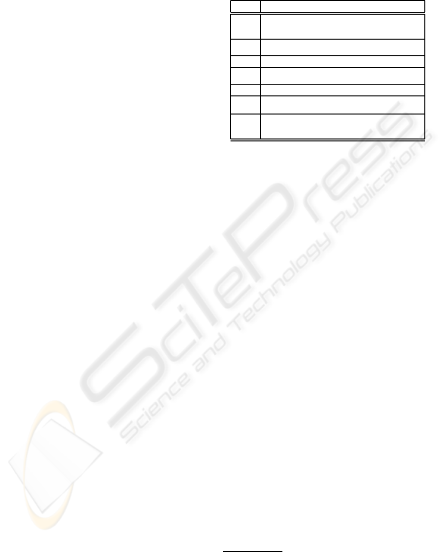
Table 2: One-Minute Microwave Oven Requirements.

Req. Description

There is a single control button available for the use of the oven.

If the oven is closed and you push the button, the oven will start

cooking (that is, energise the power-tube) for one minute.

If the button is pushed while the oven is cooking, it will cause the

oven to cook for an extra minute.

Pushing the button when the door is open has no effect.

Whenever the oven is cooking or the door is open, the light in the

oven will be on.

Opening the door stops the cooking.

Closing the door turns off the light. This is the normal idle state,

prior to cooking when the user has placed food in the oven.

If the oven times out, the light and the power-tube are turned off

and then a beeper emits a warning beep to indicate that the cook-

ing has ﬁnished.

4 A CLASSICAL EXAMPLE

We proceed here to illustrate our approach with an ex-

ample that has been repeatedly used by the software

engineering community, e.g. (Dromey and Powell,

2005; Myers and Dromey, 2009; Shlaer and Mellor,

1992; Wen and Dromey, 2004; Mellor, 2007). This

is the so called one-minute microwave oven (Shlaer

and Mellor, 1992). Table 2 shows the requirements as

presented by Myers and Dromey (Myers and Dromey,

2009, p. 27, Table 1). Although this is in fact not

exactly the same as the original by Shlaer and Mel-

lor (Shlaer and Mellor, 1992, p. 36), we have cho-

sen the former rather than the latter because we will

later compare with Behavior Trees regarding model

size and direct code generation.

4.1 Microwave in Plausible Logic

Because we have a software architecture that handles

communication between modules through a decou-

pling mechanism named the whiteboard (Billington

et al., 2009), we can proceed at a very high level. We

assume that sensors, such as the microwave button,

are hardware instruments that deposit a message on

the whiteboard with the signature of the depositing

module and a time stamp. Thus, events like a but-

ton push or actions such as energising the microwave

tube are communicated by simply placing a message

on the whiteboard.

Thus, knowledge of an event like

a button push simply exists because a corresponding

message has appeared on the whiteboard. Similarly,

an action like energising the microwave tube is trig-

Matters are a bit more complex, as messages on the

whiteboard expire or are consumed, and for actuators, they

could have a priority and thus actuators can be organised

with “subsumption” (Brooks, 1991).

NON-MONOTONIC REASONING FOR REQUIREMENTS ENGINEERING - State Diagrams Driven by Plausible Logic

% MicrowaveCook.d

name{MicrowaveCook}.

input{timeLeft}.

input{doorOpen}.

C0: {} => ˜cook.

C1: timeLeft => cook. C1 > C0.

C2: doorOpen => ˜cook. C2 > C1.

output{b cook, "cook"}.

output{b ˜cook, "dontCook"}.

(a) DPL for 2-state machine controlling

tube, fan, and plate.

% MicrowaveLight.d

name{MicrowaveLight}.

input{timeLeft}.

input{doorOpen}.

L0: {} => ˜lightOn.

L1: timeLeft => lightOn. L1 > L0.

L2: doorOpen => lightOn. L2 > L0.

output{b lightOn, "lightOn"}.

output{b ˜lightOn, "lightOff"}.

(b) DPL for 2-state machine

controlling the light.

Figure 2: Simple theories for 2-state machines.

gered by placing a different message on the white-

board. The driver for the corresponding actuator then

performs an action for this particular message as soon

as it appears on the whiteboard.

However, here the label

cook

for the transition

of the state NOT COOKING to the state COOKING and

the label

dontCook

from COOKING to NOT COOKING

are not necessarily events. They are consequents in a

logic model. For example,

dontCook

is an output of

such a model that acts as the cue to halt the cooking.

The logic model will specify the conditions by which

this cue is issued. Fig. 2a shows the logic model

in the logic programming language DPL that imple-

ments PL. In the case of the microwave oven require-

ments, for the purposes of building a model, a system

analyst or software engineer would ﬁrst identify that

there are two states for various actuators. When the

oven is cooking, the fan is operating, the tube is en-

ergised and the plate is rotating. When the oven is

not cooking, all these actuators are off. The approach

can be likened to arranging the score for an orches-

tra: all these actuators will need the same cues from

the conductor (the control) and, in this example, all

switch together from the state of COOKING to the state

of NOT COOKING and vice versa. They will all syn-

chronously consume the message to be off or to be on.

Thus, we have a simple state diagram to model this

(Fig. 3a). By default, we do not have the conditions

to cook. This is Rule

in the logic model (called a

(a) A 2-state machine for controlling

tube, fan, and plate.

(b) A 2-state machine for

controlling the light.

Figure 3: Simple 2-state machines control most of the mi-

crowave.

theory) relevant to the cooking actuators. However, if

there is time left for cooking, then we have the con-

ditions to cook (Rule

) and this rule takes priority

over

. However, when the door opens, then we do

not cook:

takes priority over

The light in the microwave is on when the door is

open as well as when the microwave is cooking. So,

the cues for the light are not the same as those for en-

ergising the tube. However, the light is in only one of

two states LIGHT OFF or LIGHT ON. The default state

is that the light is off. This is Rule

in the theory for

the light (see Fig. 2b). However, when cooking the

light is on. So Rule

has priority over

. There is a

further condition that overwrites the state of the light

being off, and that is when the door is open (Rule

Note that in this model, the two rules

and

over-

ride the default Rule

, while in the model for cook-

ing the priorities caused each new rule to reﬁne the

previous rule. The control button (Fig. 4) also has

two states. In one state, CB ADD, the time left can

be incremented, while in the other state, pushing the

button has no effect. Again, between these two states

we place transitions labelled by an expression of PL

(in all cases, simple outputs of a theory). The control

button does not add time unless the button is pushed.

This is reﬂected by Rule

CB0

and Rule

CB1

below and

the priority that

CB1

has over

CB0

. When the door

is open, pushing the button has no effect; this is Re-

quirement R3 and expressed by Rule

CB2

and its pref-

erence over

CB1

. Because we already have deﬁned

that a push of a button adds time to the timer (except

for the conditions already captured), if the button is

not pushed, then we do not add time. This is a strict

rule that in DPL is expressed by a disjunction.

The ﬁnal requirement to model is the bell, which

is armed while cooking, and rings when there is no

time left. This is the transition

noTimeLeft

from

ENASE 2010 - International Conference on Evaluation of Novel Approaches to Software Engineering

(a) State machine

% MicrowaveButton.d

name{MicrowaveButton}.

input{doorOpen}.

input{buttonPushed}.

CB0: {} => ˜add.

CB1: buttonPushed => add. CB1 > CB0.

CB2: doorOpen => ˜add. CB2 > CB1.

\/{buttonPushed, wait}.

output{b add, "add"}.

output{b wait, "wait"}.

(b) DPL theory

Figure 4: The modelling of the button’s capability to add to

the timer.

(a) Bell state machine

% MicrowaveBell.d

name{MicrowaveBell}.

input{timeLeft}.

output{b ˜timeLeft, "noTimeLeft"}.

(b) DPL theory for the bell.

Figure 5: The modelling of the bell’s capability to ring when

the time expires.

BELL ARMED to BELL RINGING in Fig. 5. After ring-

ing, the bell is off, and when cooking time is added

to the timer, it becomes armed. The logical model is

extremely simple, because the condition that departs

from BELL ARMED to BELL RINGING is the negation of

the one that moves from to BELL OFF to BELL ARMED.

Moreover, we always move from BELL RINGING to

BELL OFF. The most important aspect of this approach

is that this is all the software analysis required in or-

der to obtain the working program.

#define dontCook ( \

doorOpen \

|| !timeLeft \

)

#define cook ( \

!doorOpen && timeLeft \

)

(a) Tube, fan and plate

#define lightOff ( \

!doorOpen && !timeLeft \

)

#define lightOn ( \

doorOpen \

|| timeLeft \

)

(b) The light

#define add ( \

buttonPushed && !doorOpen \

)

#define wait ( \

!buttonPushed \

)

#define noTimeLeft ( \

!timeLeft \

)

(d) The bell

Figure 6: Translated C expressions for transitions.

4.2 Translation into Code

Once the high level model has been established in

DPL, translation into code is straightforward. A

Haskell proof engine implementation of DPL allows

the interpretation and formal veriﬁcation of the devel-

oped rule sets (Billington and Rock, 2001). This im-

plementation was extended to include a translator that

generates code that can be used in C, C++, Objective-

C, C# and Java. The Haskell translator creates op-

timised Boolean expressions through the truth tables

generated from the DPL rules. These Boolean ex-

pressions are then written out as C code that can di-

rectly be compiled and linked with libraries and appli-

cation code. Incidentially, the C syntax for Boolean

expressions is not only the same in supersets of C

(such as C++ and Objective-C), but also in modern,

related programming languages such as Java

Figure 6 shows the DPL theories for the state dia-

gram transitions translated into C by the Haskell proof

engine. This code can then directly be used as a

header ﬁle for a generic embedded system state ma-

chine to test the transition conditions. Subsequent re-

ﬁnements of the rules do not require any changes to

the generic state machine code. A simple recompila-

tion against the updated, generated header ﬁles is suf-

ﬁcient to update the behaviour of the state machine.

5 EVALUATION

The original approaches to modelling behaviour with

ﬁnite state diagrams (Rumbaugh et al., 1991; Shlaer

At this stage, expressions are generated using the

#define

preprocessor syntax, that is not supported directly

in Java, but can easily be extracted using a script or even

copy and paste.

NON-MONOTONIC REASONING FOR REQUIREMENTS ENGINEERING - State Diagrams Driven by Plausible Logic

and Mellor, 1992) had little expectation that the mod-

els would directly translate to implementations with-

out the involvement of programmers using imperative

object-oriented programming languages. However,

the software development V-model (Wiegers, 2003)

has moved the focus to requirements modelling, and

then directly obtaining a working implementation, be-

cause this collapses the requirements analysis phase

with the veriﬁcation phase. There are typically two

approaches. First, emulating or simulating the model,

which has the advantage that software analysts can

validate the model and implementation by running

as many scenarios as possible. The disadvantage is

the overhead incurred through the interpretation of

the model, rather than its compilation. The second

approach consists of generating code directly from

the model (Wagner and Wolstenholme, 2003; Wagner

et al., 2006). This removes the overhead of interpret-

ing at run-time the modelling constructs. Approaches

to the automatic execution or translation of models

for the behaviour of software have included the use

of UML state diagrams for generating code (Mellor,

2007), the automatic emulation or code generation

from Petri nets (Girault and Valk, 2001), and the au-

tomatic emulation or code generation from Behavior

Trees (Wen and Dromey, 2004; Wen et al., 2007b;

Wen et al., 2007a). A more recent trend is mod-

els@run.time, where “there is a clear pressure arising

for mirroring the problem space for more declarative

models” (Blair et al., 2009).

5.1 Contrast with State Diagrams

Simulation and direct generation of code from a state

diagram is clearly possible, since one only needs to

produce generic code that reads the transition table

(encoded in some standard form), then deploy and

interpret that repeatedly by analysing the events re-

ceived as well as the current state, and moving to the

proper subsequent state. This has been suggested for

UML (Mellor, 2007) and is the basis of the design pat-

tern

state

(Larman, 1995, p. 406). However, while

Finite State Machines continue to enjoy tremendous

success (Wagner and Wolstenholme, 2003), “there is

no authoritativesource for the formalsemantics of dy-

namic behavior in UML” (Winter et al., 2009). The

best example for the success of Finite State Machines

is stateWorks (

www.stateworks.com

) and its method-

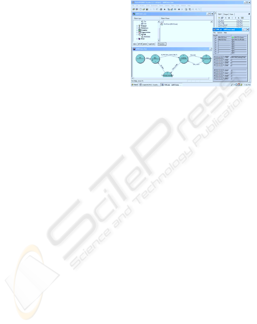
ology (Wagner et al., 2006). We have downloaded

the 60-day free license of stateWorks Studio and the

SWLab simulator (Fig. ??). Note that this ﬁnite state

machine has only 5 states (the documentation of this

example with stateWorks admits the model has is-

sues, e.g. “to reset the system for the next start, we

Figure 7: The execution of the example model provided in

the demo version of stateWorks for a microwave oven.

have to open and then close the door” and “the con-

trol system always starts even when the timeout value

is 0”). These issues can be ﬁxed but additional infras-

tructure is necessary, including ‘counters’ and ‘switch

points’ as well as usage of the ‘real time database

(RTDN)’. The stateWorks example describes generic

of microwave behaviour and needs some more polish-

ing to capture more detailed requirements e.g. those

outlined in Table 2. Since we argue in favour of us-

ing ﬁnite state machines for modelling behaviour, this

tool concurs with that approach. However, our eval-

uation conﬁrms that using PL is more powerful and

closer to the original speciﬁcation than the “positive-

logic” transitions in stateWorks.

5.2 Contrast with Petri Nets

Petri Nets (Peterson, 1977; Holloway et al., 1997)

provide a formal model for concurrency and synchro-

nisation that is not readily available in state diagrams.

Thus, they offer the possibility of modelling multi-

threaded systems that support requirements for con-

currency. Early in the modelling effort Petri Nets

were dismissed: “Although they succeed well as an

abstract conceptual model, they are too low level

and inexpressive to be useful to specify large sys-

tems” (Rumbaugh et al., 1991, p. 144). However,

because it is quite possible to simulate or interpret a

Petri Net (or to generate code directly from it), they

continue to be suggested as an approach to directly

obtain implementations from the coding of the re-

quirements (Gold, 2004; Lian et al., 2008; Lakos,

2001; Saldhana and Shatz, 2000).

We have used PIPE 2.5 (

pipe2.sf.net

) to con-

struct a model of the microwave as per the require-

ments in Table 2 (see Fig. 8). It becomes rapidly ap-

parent that the synchronisation of states between com-

ENASE 2010 - International Conference on Evaluation of Novel Approaches to Software Engineering

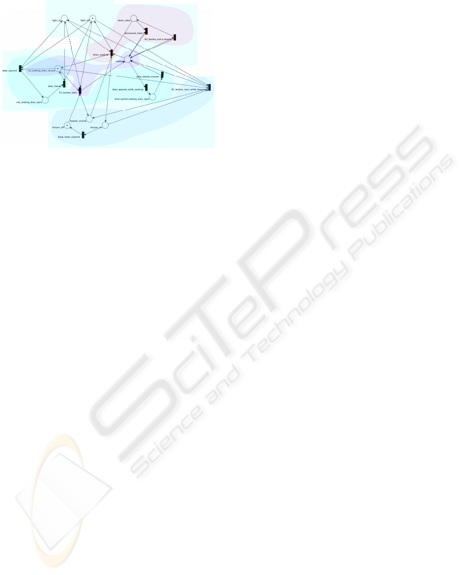
Figure 8: Capturing the requirements in Table 2 as a Petri

Net, grouped by the various components of the microwave.

ponents of the system forces to display connectors

among many parts in the layout, making the model

hard to grasp.Even if we consider incremental devel-

opment, each new requirement adds at least one place

and several transitions from/to existing places. There-

fore, we tend to agree that even for this small case

of the one-minute microwave, the Petri Net approach

seems too low level and models are not providing a

level of abstraction to assist in the behaviour engi-

neering of the system. One advantage of Petri Net

models is that there are many tools and algorithms

for different aspects of their validation. For example,

once a network is built with

PIPE

, this software has

algorithms to perform GSPN Analysis, FSM analy-

sis, and Invariant Analysis. However, even for this

example, considered simple and illustrative in many

circles, the model is not a suitable input for any of the

veriﬁcation analysis in

PIPE

. On a positive note, some

ﬁrst-order logics have been included in transitions to

create Predicate/Transition Nets (Genrich and Laut-

enbach, 1979; Genrich, 1991). Consequently, we see

no reason why our approach to use a non-monotonic

logic cannot be applied to Petri Nets.

5.3 Contrast with Behavior Trees

Behavior Trees (Wen et al., 2007a) is another pow-

erful visual approach for Behaviour Engineering (the

systematic progression from requirements to the soft-

ware of embedded systems). The approach provides

a modelling tool that constructs acyclic graphs (usu-

ally displayed as rooted tree diagrams) as well as

a Behavior Modelling Process (Dromey and Powell,

2005; Myers and Dromey, 2009) to transform nat-

ural language requirements into a formal set of re-

quirements. The Embedded Behavior Runtime En-

vironment (eBRE) (Myers and Dromey, 2009) exe-

cutes Behavior Tree models by applying transforma-

tions and generating C source code. The tool Be-

havior Engineering Component Integration Environ-

ment (BECIE) allows Behavior Trees to be drawn

and simulated. Proponents of Behavior Trees argue

that these diagrams enable requirements to be de-

veloped incrementally and that speciﬁcations of re-

quirements can be captured incrementally (Wen et al.,

2007b; Wen and Dromey, 2004). The classic exam-

ple of the one-minute microwave has also been ex-

tensively used by the Behavior Tree community (Wen

and Dromey, 2004; Dromey and Powell, 2005; Myers

and Dromey, 2009). Unfortunately, for this example,

Behavior Trees by comparison are disappointing. In

the initial phase of the method, requirements R1, R2,

R5, R6 in Table 2 use ﬁve boxes (Wen and Dromey,

2004; Dromey and Powell, 2005), while R3 and R4

demand four. Six boxes are needed for requirement

R7 (Wen and Dromey, 2004; Dromey and Powell,

2005). Then, the Integration Design Behavior Tree

(DBT) demands 30 nodes (see (Dromey and Powell,

2005, p. 9) and (Wen and Dromey, 2004, Fig. 5)). By

the time it becomes a model for eBRE the microwave

has 60 nodes and 59 links! (Myers and Dromey, 2009,

Fig. 6) and the Design Behavior Tree (Myers and

Dromey, 2009, Fig. 8) does not ﬁt legibly on an A4

page. Sadly, the approach seems to defeat its pur-

pose, because on consideration of the system bound-

aries (Myers and Dromey, 2009, Fig. 7), outputs to

the alarm are overlooked. Moreover, the language for

logic tests in the tools for Behavior Trees is far more

limited than even the ‘positive-logic’ of stateWORKS.

The equivalence between ﬁnite state machines and

Behavior Trees (Billington et al., 2010) is based on

the observation that Behavior Trees correspond to the

depth-ﬁrst search through the treads of the states of

the system behaviour control. It is not surprising that

the notion needs far more nodes and connections than

the corresponding ﬁnite state machine.

6 FINAL REMARKS

We stress two more aspects of the comparison. First,

the approaches above attempt, in one way or another,

to construct the control unit of the embedded system,

and from it the behaviour of all of its components.

This implies that the control unit has a state space

that is a subset of the Cartesian product of the states

of the components. Our approach is more succinct

not only because of a more powerful logic to describe

state transition, but because our software architecture

decouples control into descriptions for the behaviour

of components. Second, our experience with this ap-

proach and the development of non-monotonic mod-

NON-MONOTONIC REASONING FOR REQUIREMENTS ENGINEERING - State Diagrams Driven by Plausible Logic

Figure 9: Hardware running Java generated code.

els show that capturing requirements is structured and

incremental, enabling iterative reﬁnement. That is,

one can proceed from the most general case, and pro-

duce rules and conditions for more special cases. We

ensured that our method delivers executable embed-

ded systems directly from the modelling by imple-

menting an oven where the hardware is constructed

from LEGO Mindstorm pieces, sensors, and actuators

(see Fig. 9). As with eBRE, we output Java source

code but execute a ﬁnite state machine. The execu-

tion then is veriﬁed because of the clear connection

between the model and the source code (as well as

testing it on the hardware).

REFERENCES

Antoniou, G. (1997). Nonmonotonic Reasoning. MIT Press,

Cambridge, Mass. ISBN 0-262-01157-3.

Billington, D. (2008). Propositional clausal defeasible

logic. In Holldobler, S., Lutz, C., and Wansing,

H., editors, Logics in Artiﬁcial Intelligence, volume

5293 of Lecture Notes in Artiﬁcial Intelligence, pages

34–47, Dresden, Germany. 11th European Confer-

ence on Logics in Artiﬁcial Intelligence (JELIA2008),

Springer.

Billington, D., Estivill-Castro, V., Hexel, R., and Rock,

A. (2009). Architecture for hybrid robotic behavior.

In Corchado, E., Wu, X., Oja, E., Herrero, A., and

Baruque, B., editors, 4th International Conference on

Hybrid Artiﬁcial Intelligence Systems HAIS, volume

5572, pages 145–156. Springer-Verlag Lecture Notes

in Computer Science.

Billington, D., Estivill-Castro, V., Hexel, R., and Rock, A.

(2010). Plausible logic facilitates engineering the be-

havior of autonomous robots. In Proceedings of the

IASTED Software Engineering Conference.

See www.youtube.com/watch?v=iEkCHqSfMco for

the system in operation. The corresponding Java sources

and incremental Petri net stages for Fig. 8 are at vladestivill-

castro.net/additions.tar.gz as well as material from (Billing-

ton et al., 2010).

Billington, D. and Rock, A. (2001). Propositional plausible

logic: Introduction and implementation. Studia Log-

ica, 67:243–269. ISSN 1572-8730.

Blair, G., Bencomo, N., and Frnce, R. B. (2009). Mod-

els@run.time. IEEE Computer, 42(10):22–27.

Brooks, R. (1991). Intelligence without reason. In My-

opoulos, R. and Reiter, R., editors, Proceedings of

the 12th International Joint Conference on Artiﬁcial

Intelligence, pages 569–595, San Mateo, CA. ICJAI-

91, Morgan Kaufmann Publishers. Sydney, Australia.

ISBN 1-55860-160-0.

Compton, P. and Jansen, R. (1990). A philosophical basis

for knowledge acquisition. Knowledge Acquisition,

2(3):241–257. ISSN 0001-2998.

Dromey, R. G. and Powell, D. (2005). Early requirements

defect detection. TickIT Journal, 4Q05:3–13.

Ellis, C. (1997). Team automata for groupware systems. In

GROUP ’97: Proceedings of the international ACM

SIGGROUP conference on Supporting group work,

pages 415–424, New York, NY, USA. ACM.

Genrich, H. J. (1991). Predicate/transition nets. In

Jensen, K. and Rozenberg, G., editors, High-level

Petri Nets, Theory and Applications, pages 3–43.

Springer-Verlag.

Genrich, H. J. and Lautenbach, K. (1979). The analysis of

distributed systems by means of predicate/transition-

nets. In Kahn, G., editor, Semantics of Concurrent

Computation, Proceedings of the International Sym-

posium, volume 70 of Lecture Notes in Computer Sci-

ence, pages 123–147, Evian, France. Springer.

Girault, C. and Valk, R. (2001). Petri Nets for System Engi-

neering: A Guide to Modeling, Veriﬁcation, and Ap-

plications. Springer-Verlag New York, Inc., Secaucus,

NJ, USA.

Gold, R. (2004). Petri nets in software engineering. Arbeits-

berichte Working Papers. Fachhochschule Ingolstadt,

University of Applied Sciences.

Holloway, L., Kroch, B., and Giua, A. (1997). A survey

of Petri net methods for controlled discrete event sys-

tems. Discrete Event Dynamic Systems: Theory and

Applications, 7:151–190.

Hull, E., Jackson, K., and Dick, J. (2005). Requirements

Engineering. Springer, USA, second edition.

Lakos, C. (2001). Object oriented modeling with object

petri nets. In Agha, G., de Cindio, F., and Rozen-

berg, G., editors, Concurrent Object-Oriented Pro-

gramming and Petri Nets, Advances in Petri Nets,

volume 2001 of Lecture Notes in Computer Science,

pages 1–37. Springer.

Larman, C. (1995). Applying UML and Patterns: An In-

troduction to Object-Oriented Analysis and Design

and Iterative Development. Prentice-Hall, Inc., En-

glewood Cliffs, NJ.

Lian, J., Hu, Z., and Shatz, S. M. (2008). Simulation-based

analysis of UML statechart diagrams: Methods and

case studies. The Software Quality Journal, 16(1):45–

78.

ENASE 2010 - International Conference on Evaluation of Novel Approaches to Software Engineering

Mellor, S. J. (2007). Embedded systems in UML. OMG

White paper. www.omg.org/news/whitepapers/ label:

We can generate Systems Today.

Myers, T. and Dromey, R. G. (2009). From requirements

to embedded software - formalising the key steps.

In 20th Australian Software Engineering Conference

(ASWEC), pages 23–33, Gold Cost, Australia. IEEE

Computer Society.

Nuseibeh, B. and Easterbrook, S. M. (2000). Requirements

engineering: a roadmap. In ICSE - Future of SE Track,

pages 35–46.

Peterson, J. L. (1977). Petri nets. Computer Surveys,

9(3):223–252.

Rumbaugh, J., Blaha, M. R., Lorensen, W., Eddy, F., and

Premerlani, W. (1991). Object-Oriented Modelling

and Design. Prentice-Hall, Inc., Englewood Cliffs,

NJ.

Russell, S. and Norvig, P. (2002). Artiﬁcial Intelligence:

A Modern Approach. Prentice-Hall, Inc., Englewood

Cliffs, NJ, second edition. ISBN 0130803022.

Saldhana, J. A. and Shatz, S. M. (2000). Uml diagrams

to object petri net models: An approach for mod-

eling and analysis. In International Conference on

Software Engineering and Knowledge Engineering

(SEKE), pages 103–110, Chicago.

Shlaer, S. and Mellor, S. J. (1992). Object lifecycles : mod-

eling the world in states. Yourdon Press, Englewood

Cliffs, N.J.

ter Beek, M., . Ellis, C., Kleijn, J., and Rozenberg, G.

(2003). Synchronizations in team automata for group-

ware systems. Computer Supported Cooperative Work

(CSCW), 12(1):21–69.

Wagner, F., Schmuki, R., Wagner, T., and Wolstenholme,

P. (2006). Modeling Software with Finite State Ma-

chines: A Practical Approach. CRC Press, NY.

Wagner, F. and Wolstenholme, P. (2003). Modeling and

building reliable, re-useable software. In Engineer-

ing of Computer-Based Systems (ECBS-03), IEEE In-

ternational Conference on the, pages 277–286, Los

Alamitos, CA, USA. IEEE Computer Society.

Wen, L., Colvin, R., Lin, K., Seagrott, J., Yatapanage, N.,

and Dromey, R. (2007a). “Integrare”, a collaborative

environment for behavior-oriented design. In Luo, T.,

editor, Cooperative Design, Visualization, and Engi-

neering, 4th International Conference, CDVE, volume

4674 of Lecture Notes in Computer Science, pages

122–131, Shanghai, China. Springer.

Wen, L. and Dromey, R. G. (2004). From requirements

change to design change: A formal path. In 2nd In-

ternational Conference on Software Engineering and

Formal Methods (SEFM 2004), pages 104–113, Bei-

jing, China. IEEE Computer Society.

Wen, L., Kirk, D., and Dromey, R. G. (2007b). A tool to vi-

sualize behavior and design evolution. In Di Penta, M.

and Lanza, M., editors, 9th International Workshop

on Principles of Software Evolution (IWPSE 2007),

in conjunction with the 6th ESEC/FSE joint meeting,

pages 114–115, Dubrovnik, Croatia. ACM.

Wiegers, K. E. (2003). Software Requirements. Microsoft

Press, second edition.

Winter, K., Colvin, R., and Dromey, R. G. (2009). Dy-

namic relational behaviour for large-scale systems.

In 20th Australian Software Engineering Conference

(ASWEC 2009), pages 173–182, Gold Cost, Australia.

IEEE Computer Society.

Wooldridge, M. (2002). An Introduction to MultiA-

gent Systems. John Wiley & Sons, NY, USA.

ISBN 047149691X.

NON-MONOTONIC REASONING FOR REQUIREMENTS ENGINEERING - State Diagrams Driven by Plausible Logic