USING MODELICA MODELLING LANGUAGE FOR PHYSICAL
PLANT PARAMETERS EVALUATION AND OPTIMIZATION
A Case Study
Eurico Seabra and José Machado
Department of Mechanical Engineering, CT2M Research Center, University of Minho, 4800-058 Guimarães, Portugal
Keywords: Modeling, Simulation, Modelica Modeling Language, Hybrid Plants, Dependable Controllers.
Abstract: Modelica Modeling language is powerful and suitable for modeling mechatronic systems, being possible to
interact different technological aspects and deal, simultaneously with different technologies (mechanical,
electrical, pneumatic, hydraulic,..). In this paper it is discussed, in a case study, the possibility of using this
language for modeling an automation system (controller and plant) in closed loop behavior and also in
defining some parameters of the automation system in order to optimize some behavior aspects of the
system as, for instance, the time cycle of the automation system. Some aspects relied with controllers
dependability are also discussed and it is showed how Modelica modeling language can help controllers’
designers improving controllers dependability, when are used Simulation Techniques.
1 INTRODUCTION
There is a rapidly increasing use of computer
simulations in industry to optimize products, to
reduce product development costs and time by
design optimization, and to train operator. Whereas
in the past it was considered sufficient to simulate
subsystems separately, the current trend is to
simulate increasingly complex physical systems
composed of subsystems from multiple domains.
In such a complex industrial process, simulation
tools are extremely useful since they can contribute
to higher product quality and production efficiency
in several ways. For example, modifications in a
plant could be tested (both statistically and
dynamically) in advance in a simulator saving much
of the trial and error procedure that is used
nowadays; the optimization of plant behavior
parameters can be performed too. Besides, a
dynamic simulator of the plant and of its control
would allow for a thorough study of different control
strategies, and would be an efficient way to tune
controllers for new equipments. Finally, a simulation
tool can also be a way of training not only the
operators but also the production engineers and
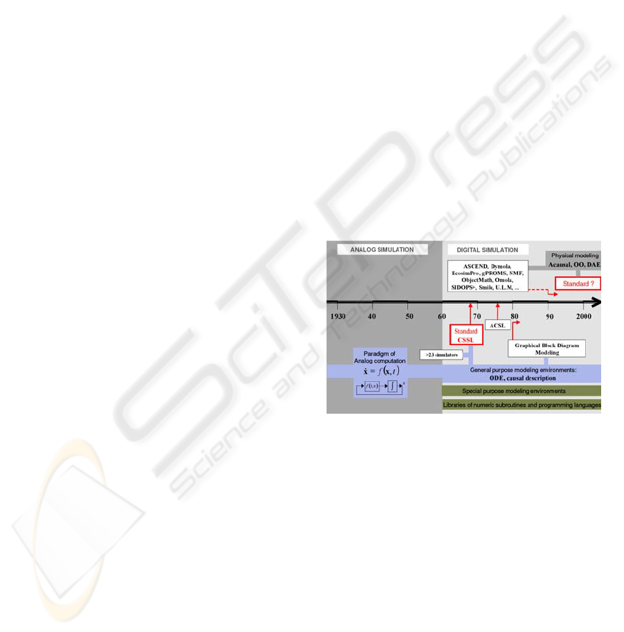
technicians. Some tools have been developed in
order to simulate the behavior of automation systems
(figure 1).
Figure 1: Evolution of modeling and simulation tools.
Graphical block diagram modeling is widely
used in control engineering (Karayanakis, 1995).
Some examples of languages and environments
supporting this paradigm are Matlab/Simulink
(Matlab, 2010), MATRIXX/SystemBuild (Matrixx,
2010), HYBRSIM (Mosterman, 2002) and ACSL
Graphics Modeller (MGA Software 1996). Block
diagram modeling paradigm might be considered as
a heritage of analog simulation (Aström et al. 1998).
On the other hand, object-oriented modeling
languages and compilers supporting the physical
modeling paradigm have become available since the
1990’s decade. This is driven by demands from
users to be able to simulate complex multi-domain
models.
199
Seabra E. and Machado J. (2010).
USING MODELICA MODELLING LANGUAGE FOR PHYSICAL PLANT PARAMETERS EVALUATION AND OPTIMIZATION - A Case Study .
In Proceedings of the 7th International Conference on Informatics in Control, Automation and Robotics, pages 199-205
DOI: 10.5220/0003005301990205
Copyright
c
 SciTePress

In this paper it is presented a study and shown
how Modelica modeling language can be used to
optimize plant behavior parameters in order to
guarantee the good and desired behavior for the
system, in the shorter time cycle, combined with
other aspects like energy consumption, for example.
To achieve the proposal goal, the section 2 is
devoted to the presentation of Modelica modeling
language and the Dymola Simulation environment;
section 3 presents the case study that is the base for
our study; section 4 discusses the mathematical
modeling of the plant. Further, section 5 presents the
Modelica model of the system (controller model
coupled with plant model); section 6 discusses the
obtained results concerning the defined plant
behavior parameters to study and, finally, section 7,
presents some conclusions and future works, in this
field.
2 MODELICA AND DYMOLA
In the few years of research in modeling and
simulation, the concept of object-oriented modeling
has achieved a big relevance. Several works have
demonstrated how objected oriented concepts can be
successfully employed to support hierarchical
structuring, reuse and evolution of large and
complex models independent from the application
domain and specialized graphical formalism.
To handle complex models, the reuse of standard
model components is a key issue. But in order to
exchange models between different packages an
unified language is needed. Modelica is an object-
oriented, general-purpose modeling language that is
under development in an international effort to
introduce an expressive standardized modeling
language, see (Elmqvist and Mattson, 1997)
(Fritzson and Vadim, 1998). Modelica supports
object-oriented modeling using inheritance concepts
taken from computer languages such as Simula and
C++. It also supports non-causal modeling, meaning
that model’s terminals do not necessarily have to be
assigned an input or output role. In fact, in the last
few years it has been proved in several cases that
non-causal simulation techniques perform much
better than the ordinary object-oriented tools.
Modelica is a powerful programming language
where equations are used for modeling of the
physical phenomena. No particular variable needs to
be solved for manually because the software Dymola
(Dymola software, 2010) has enough information to
decide that automatically. This is an important
property of Dymola to enable handling of large
models having more than hundred thousand
equations. Modelica supports several formalisms:
ordinary differential equations (ODE), differential-
algebraic equations (DAE), bond graphs, finite state
automata, Petri nets, etc.
3 CASE STUDY DESCRIPTION
The case study that is proposed as base for this work
is inspired on the benchmark system proposed by
(Kowalewski et al. 2001).
Figure 2 illustrates an example of an evaporator
system, which consists of two tanks, where an
aqueous solution suffers transformations. In the first
tank that solution should acquire a certain
concentration through the heating of the solution
using an electrical resistance (H1) which provokes
the steam formation.
Associated to the tank1 (figure 2) exist a
condenser (C) responsible for the condensation of
the steam that however it was formed. The cooling,
in that condenser, it is done through the circulation
of a cooling liquid (whose flow is measured by
sensor FIS) that passes through the cooling circuit (if
open the valve V13).
Associate to the tank1 there are a group of
sensors: level sensors (maximum (LIS1) and
minimum (LII1)), temperature sensor (acceptable
maximum (TIS1)); sensor of conductivity (QIS) that
is to indicate the desired concentration; they also
exist several actuators: filling valve of the tank1
(V12), drain valve (V16) and emptying valve (V15),
that it is also the filling valve of the tank2.
Figure 2: Scheme of the entire evaporator system.
In the normal operation mode, the system works
as follows.
The tank1 should be previously filled to its
superior level with an aqueous solution by opening
valve V12. When the tank1 is full, the heating
ICINCO 2010 - 7th International Conference on Informatics in Control, Automation and Robotics
200

system is switch on and also, in simultaneous, the
cooling system of the condenser by opening valve
V13. When it is formed steam, this condenses in the
condenser C. When the concentration desired in the
tank1 is reached, there are switch off the heating
system and the cooling system of the condenser.
Continuously the solution flows from tank1 into
tank2, and it must be guaranteed that the tank2 is
empty. The transfer of the solution to the tank2 is for
a powder-processing operation that is not, here,
described. For that powder-processing operation,
there is necessary to heat the solution to avoid
possible crystallization, and for that there are two
approaches: it can heat until the temperature sensor
of the tank2 indicates that the desired temperature
was reached; or it can heat up for a certain time.
Finally, the tank2 is emptied by the pump P1, if the
valve V18 be opened.
On the other hand, in the possible failure
operation mode, the system works as follows.
A possible failure scenario of the system happens
when the cooling fluid flow in the condenser be to
low (detected by sensor FIS). This implicates the
increase of pressure and temperature in condenser C
and tank1, if the heating system keep switch on
(solution steam). It is necessary to guarantee that the
pressure in the condenser C doesn't exceed a
maximum value to avoid its explosion. For that, it
should be guaranteed that the heating in the tank1 is
switch off before the open of the safety valve (V16).
For this situation of failure operation, it should
switch off the resistance H1 the more quickly
possible, but tends in account that the solution
doesn't crystallize, then that we are before a critical
time. To switch off the resistance H1 they are
considered two possibilities: through a time after
sensor FIS to have detected reduced flow; or through
the sensor of temperature TIS1 (due to the pressure
and temperature are parameters that are directly
related).
There are evidences that should be guaranteed, as
for instance that the tanks should never overflow.
After the failure situation occurs, all of the valves
should be immediately closed.
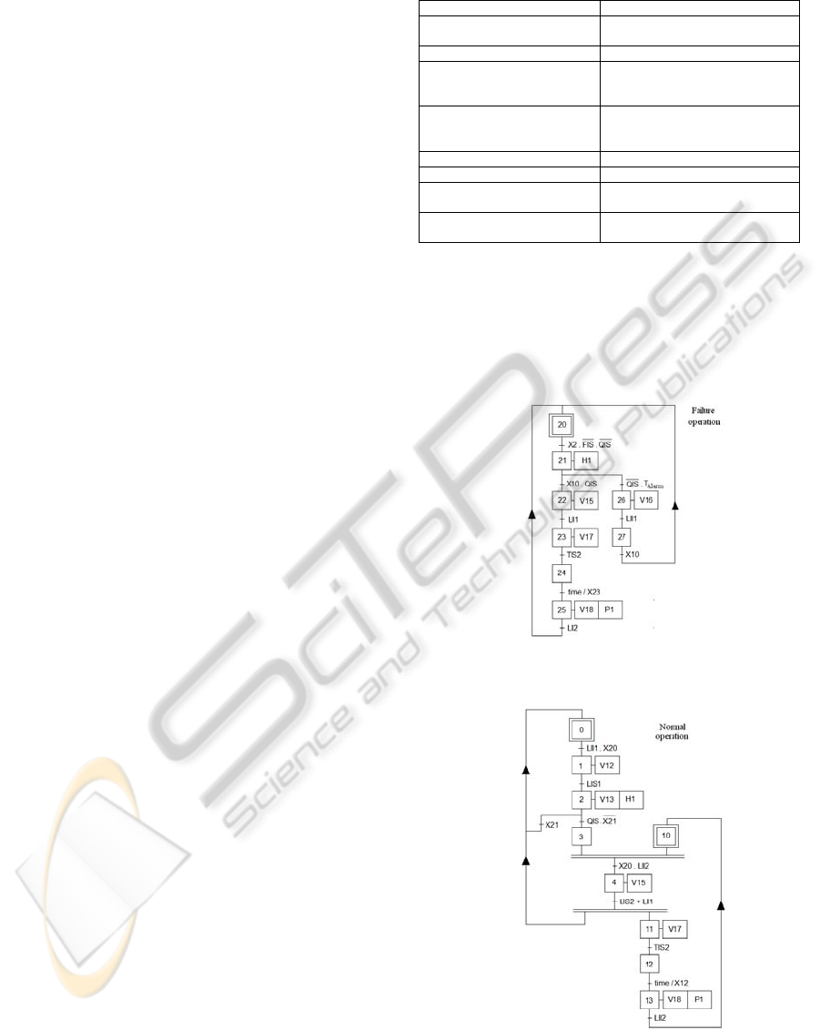
3.1 Controller Specification
In order to guarantee the desired behavior, the
controller specification was developed according to
IEC 60848 SFC specification.
Table 1: Input/Output variables of the controller.
Inputs Outputs
LIS1 – Superior level of the
tank1
V12 – Solution entrance of the tank1
LII1 – Inferior level of the tank1 V13 – Cooling of the condenser
QIS – Electrical conductivity of
the solution in tank1
(concentration)
V15 – Valve of solution passage of
the tank1 for the tank2
TAlarm– Maximum solution
temperature in tank1
(sensor T1S1)
V16 – Drain of the tank1
LIS2 – Superior level of tank2 V17 – Heating of the tank2
LII2 – Inferior level of tank2 V18 – Emptying of the tank2
TIS2 – Solution temperature in
tank2
P1 – Emptying pump of the tank2
FIS – Cooling solution flow of
the condenser C
H1 – Heating Resistance of the tank1
The input and output variables of the controller
which controls the process in closed-loop are
presented and described in table 1.
The SFC specification of the controller behavior
(normal and failure modes) is presented in figures 3
and 4.
Figure 3: SFC specification of the Controller – Normal
Operation Mode.
Figure 4: SFC specification of the Controller – Failure
Operation Mode.
USING MODELICA MODELLING LANGUAGE FOR PHYSICAL PLANT PARAMETERS EVALUATION AND
OPTIMIZATION - A Case Study
201

The controller specification was directly translated
to Modelica modeling language, more specifically to
the library for hierarchical state machines
StateGraph (Otter et al. 2005).
4 PLANT MATHEMATICAL
MODELLING
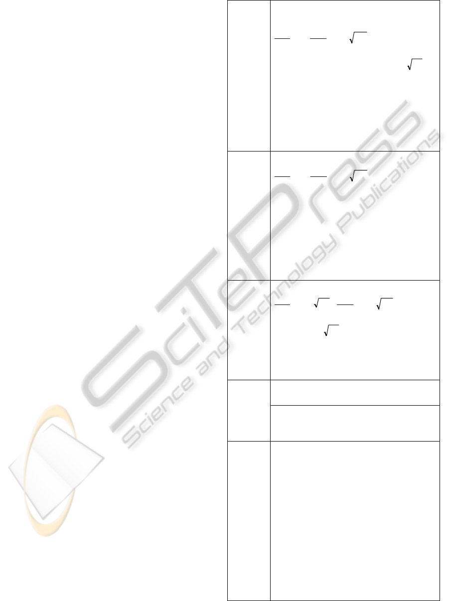
The next table presents the mathematical equations
that model the system.
The plant modelling has two goals (table 2): first
to assure that the controller specification is adequate
for the intended system behaviour and, second, to
minimize the cycle time for repetitive automation
systems processes. In this paper there are discussed
the two of them: to be sure that the system behaves
as expected – without leading to dangerous
situations - and to maximize the productivity of the
process that it implicates the maximization of the
number of batches.
Due to discrete switching between the two
different continuous systems (T1 and T2), which
happens not only at the stage transitions, by
changing the position of the on/off valves (V15 and
V18), but also in stage 2 for boiling water point, this
developed model is of hybrid nature. The main
required parameters and algebraic equations are
presented in detail in the table 2.
The setting of alarm temperature T
Alarm
is chosen
correctly to accomplish the following two opposed
very important properties: On the one hand it must
be low enough to avoid a dangerous temperature and
pressure values, and on the other hand it has to be
sufficient high so that temperature T does not fall
below a crystallization temperature before liquid
level in tank1 (H
1
) becomes zero.
5 MODELICA MODEL OF THE
SYSTEM
Due to the described potentialities, it was developed
a global model of the evaporator system, already
presented in the previous sections. The plant was
modeled as the controller using the Dymola software
and the object-oriented programming language
Modelica (Fritzson and Vadim, 1998, Elmqvist and
Mattson, 1997). Additionally, to model the
controller, it was used the library for hierarchical
state machines StateGraph (Otter et al. 2005), which
are included in the Dymola software.
Table 2: System description (differential and algebraic
equations).
Stage 1
Heating
while
T2 is
drained
EvapLossHeat
QQQdtdQ −−=)/(
dtmmcTddtdQ
VLLp
/)).(.()/(
,
+=
0
1
=
dt
dH
;
21
2
HK
dt
dH
−=
)
.(
eLoss
TTkAQ −=
dtdmQ Δ= )./(
evVEvap
h ;
gAAK
R
2)./(
21
=
2
TaTaap ++=
2
1
0
(boiling pressure, dissolve
substance ignored)
TRMmpV
mLVV
)/(=
mmm +=
;
Tbbh
ev 21
+=Δ
VLtotal
QHeat
= 6 kg (total mass of fluid),
(heat supply rate)
3
02.0 mV
V
=
KWkA /24
(vapor volume, assumed to be constant),
=
(heat loss flow per Kelvin)
Stage 2
Cooling
while
T2 is
drained
EvapLoss
QQdtdQ −−=)/(
0
1
=
dt
dH
;
21
2
HK
dt
dH
−=
T < 373K:
dtmcTddtdQ
LLp
/)..()/(
.,
=
0≅
Evap
Q
,373KT >
dtdQ
)/( =
Evap
dmQ = (
WkA 5.22
;
;
:1barp >
cTd
Lp
.(.(
.,
V
hdt Δ)./
K/
dtmm
VL
/))+
ev
.(
Loss
kAQ =
)e
TT −
=
(heat loss flow per Kelvin)
Note: In this stage it will be used the same
algebraic equations and parameters as in stage 1.
Stage 3
Cooling
while
T1 is
drained
Loss
QdtdQ −=)/(
1
2
1
HK
dt
dH
−=
;
11
2
HK
dt
dH
−=
dtmdTcdtdQ
LLp
/)/.()/(
.,
= ;
)
.(
eLoss
TTkAQ −=
gAAK
R
2)./(
12
=
;
;
11
AH
L
m
L
ρ =
11
.DHAA π +=
2
//150 mKWk = (heat loss transfer coefficient),
=0.03m
2
, =0.06m
2
(cross-sectional area T1 and
T2)
1
A
2
A
Variables
state: T (temperature in T1), , (liquid heights,
tanks considered empty when )
1
H
H
2
/
1
2
H
.0≤ m0017
algebraic: (liquid mass), (vapor mass),
L
m
hΔ
V
m
(evaporation enthalpy),
ev
p
(pressure),
A (heat loss area)
Additional
parameters
1
1T
1
a =
a
A
onstants),
kg/K
heat
(diameter of T1), gravity
nt),
=0.03m2, =0.06m
2
(cross-sectional areas of
and ), (pipe cross-sectional
area)
a ,
,
2
A
A
R
3.9 ⋅
4
10⋅
/ mN
2T
0
=
28.5−
4.75
25
10.2 m
−
=
26
/10 mN
22
// KmN
22
/ K ,,aa
2
kgJ /10
6
⋅ ,
(enthalpy constant),
c
p,
= ( pressure c
b 294.3
1
=
L
(liquid
capacity),
mD 2.0=
2
10
a
2
78.2−=b
J /4220
=
3
10⋅ J/
Kkg /
2
/81.9 smg = (
ol (molecular
iquid
nsta
constant),
M
L
314.
KT
e
283=
mkg
L
/018.0= weight of
liquid),
ρ density),
R
m
8= (molecular gas co
temperature)
3
/970 mkg= (l
molkgJ //
(environment
ICINCO 2010 - 7th International Conference on Informatics in Control, Automation and Robotics
202

Related with the odeled the
fil
plant part, it was m
ling source, the tank1 and tank2, the heater (H1),
the condenser and the valves. For that, it were used
the parameters and algebraic equations presented in
the table 2.
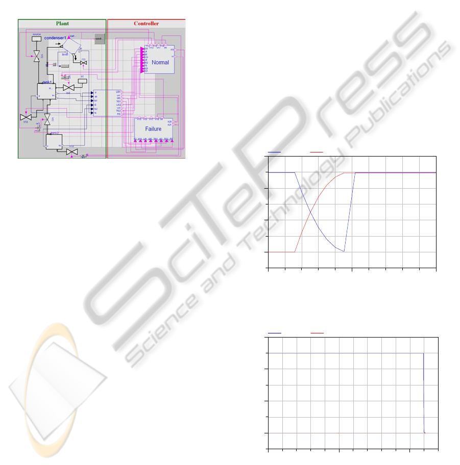
Figure 5 shows the global modelica model of the
system, being highlighted the two main parts, the
physical part (plant) on the left, and the controller on
the right. On the other hand, the controller model
was developed according the SFC specifications (see
figures 3 and 4).
Figure 5: Global modelica model of the evaporator
ue to the reason of it being specified a
di
6 SIMULATION RESULTS
ults of
was necessary to
de
of the controller system (see
fig
ns, respectively, relating to the normal
op
system.
Also, d
screte controller to control the hybrid plant, it was
necessary to implement an appropriate interface, that
translate the analogue outputs signals of the plant
(tanks levels, temperatures, concentration,…) digital
signals, that can be used as inputs of the discrete
controller.
In this section, there are presented res
simulations that were accomplished with the purpose
of studying the dynamical behavior of the hybrid
models described in the previous sections in order to
maximize the productivity of the evaporator process,
in terms, of their energy efficiency and batches
times.
Moreover, these simulations can be seen as a
“system preliminary analysis” to check if the system
behaves in agreement to a given specification for a
particular case, like as, a given a initial state of the
process and a given control program. However, it
must to be enhanced that this is not verification in
the strict sense, since it relies on the appropriate
selection of the considered cases.
In order to perform the hybrid model simulation
with different heating power’s it
fine the parameters, start and stop time of the
simulation, the interval output length or number of
output intervals and the integration algorithm. In the
present work, in all simulations performed, the Dass
algorithm (Basu et al. 2006) with 10000 output
intervals was used.
The first simulations performed was devoted to
verify if the SFC
ures 3 and 4) modeled with Modelica language
with the library for hierarchical state machines
StateGraph simulated correctly the evaporator
system.
Figures 6 and 7 show the results of the first two
simulatio
eration and failure operation modes for the level
tanks. The failure mode it is consequence of the
occurrence of the condenser malfunction during the
production cycle that it originates that the solution
temperature in the tank1 reach the alarm temperature
pre-defined (390K).
2990 3000 301
0
0.0
0.4
0.8
1.2
Fill tank [%]
Time [s]
level_tank1 level_tank2
Figure 6: Level tanks in function of time in normal
operation mode of the evaporator system.
0 1000 2000
0.0
0.4
0.8
1.2
Fill tank [%]
Time [s]
level_tank1 level_tank2
Figure 7: Level tanks in function of time in failure
operation mode of the evaporator system.
USING MODELICA MODELLING LANGUAGE FOR PHYSICAL PLANT PARAMETERS EVALUATION AND
OPTIMIZATION - A Case Study
203

Observing Figure 6 it can be concluded that the
normal operation mode is properly simulated by the
developed program, since the two main properties
that are important to prove are confirmed, for
instance, the drainage of the solution present in the
tank 1 only to happen when the tank2 is empty and
also the filling of the tank1 to happen soon after this
to be empty. On the other hand, observing figure 7,
it can be also concluded that the failure operation
mode is properly simulated, given that is proven that
the tank1 is drained through the safety valve (V16 –
see figure 2) because it is seen that the tank2
remains empty.
After being concluded that the normal and failure
operation behavior is properly simulated by the
proposed program they were performed other
simulations in order to obtain the relationship
between several physical plant parameters that can
obtain the best ratio between the number of batches
and the supply energy costs.
This manner, among of several physical variables
of the process (see table 2) it was chosen the heat
supply rate (Q
Heat
) because it is the most relevant
variable, that determine the rate of the steam
formation (this condenses in the condenser C) and
correspondingly, the time in that the solution present
in the evaporator (tank1) is prepared to be drained
(desired concentration reached).
The solution concentration (C) is obtained by the
following equation:
) /()(
0 VLL
mmmCC −⋅=
(1)
Where, C
0
is the initial concentration, m
L
is the
liquid mass and m
V
is the vapour mass. In addition,
in all of the performed simulations, it was assumed
concentration values of 0.01000 and 0.01003,
respectively, initial and final.
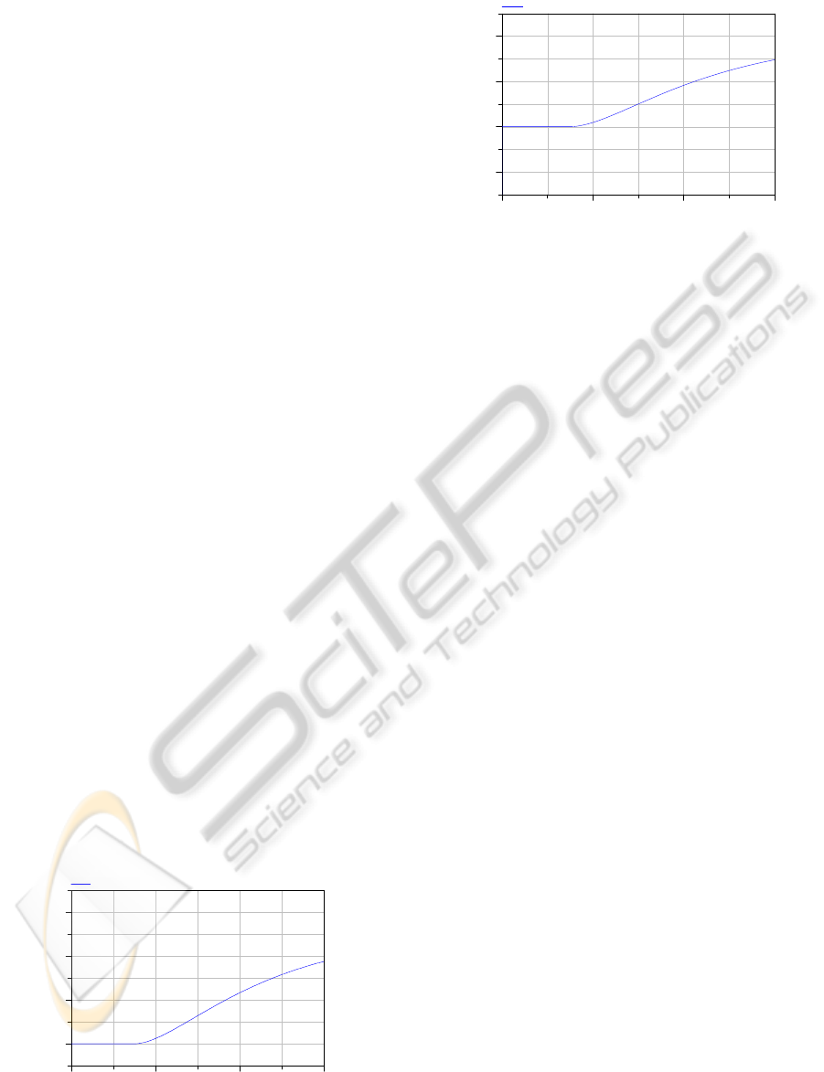
Figures 8 and 9 illustrate the behavior of the
model given in the table 2 for heat supply rate
(Q
Heat
) of 3000W, respectively for the vapour mass
and concentration.
0 1000 2000 300
0
0.00
0.01
0.02
0.03
Vapour mass [kg]
Time [s]
Vapour_tank1
Figure 8: Vapour mass in function of time with a heat
supply rate of 3000W.
0 1000 2000 300
0
0.00998
0.01000
0.01002
0.01004
Concentration
Time [s]
Concentration_tank1
Figure 9: Concentration in function of time with a heat
supply rate of 3000W.
In a general way, the results presented in the
figures 8 and 9 allow to conclude that the
concentration behavior is properly simulated by the
proposed program.
In particular, analyzing figure 8 it can be stated
that the boiling water point (373K) it is reached after
having elapsed about 800s and after this time the
vapour mass increases continually as it was foreseen
with the increase of the temperature.
On other hand, observing figure 9, it can be
verified that the time in that the solution present in
the tank1 reaches the final concentration (0.01003),
and this way prepared to be drained to tank2, is
about 3000s.
In order to be possible to generalize the batches
optimization, that it implicates the productivity
maximization of the evaporator system, it is
essential to know the optimized relation between the
heat supply rate and the time for the solution reaches
the desired concentration in the tank1 (evaporator).
Figure 10 illustrates the time for the solution
reaches the desired final concentration in function of
heat supply rate, as example, from 3000 to
100000W.
Analyzing figure 10, it can be concluded that the
increase of the heat supply rate originates a very
significant decrease on the required time for the
solution reaches the final concentration. It can be
highlighted that the more accentuated time
reductions happens in the interval from 3000 to
20000W.
This manner, in agreement with the simulations
results presented, it can be concluded that the heat
supply rate of 20000W, could be the most
appropriate to obtain the best optimization between
the number of batches and the supply energy costs,
considering the values of the physical variables of
the evaporator system presented in table 2.
ICINCO 2010 - 7th International Conference on Informatics in Control, Automation and Robotics
204

0
400
800
1200
1600
2000
2400
2800
3200
0 20000 40000 60000 80000 100000 12000
0
Heat supply rate [W]
Time [
s
Figure 10: Time for the solution present in the tank1
reaches the final concentration in function of heat supply
rate.
7 CONCLUSIONS AND FUTURE
WORK
The simulation used to evaluate the controller and
plant behavior has been developed and proposed in
this paper.
The present research proved to be successful using
the Modelica programming Language to obtain a
plant model and using it, in a closed-loop behavior,
with the controller model.
Some parameters and functional aspects of the
system have been simulated in order to define a set
of values of different variables that make the system
dependable and safe avoiding dangerous situations,
and more efficient, when studied some critical plant
behavior parameters.
The study of critical plant behavior parameters
(like presented in this paper) can be performed using
Modelica in order to obtain simulation models of
complex systems.
As future work the authors believe that, with
auxiliary calculations, it will be possible, using
simulation strategies, to define optimal values for
the different variables, in order to obtain, by one
hand, a safe system behavior and, by other hand, to
optimize the time cycle of Automation repetitive
systems taking into account the critical steps of their
functioning.
ACKNOWLEDGEMENTS
This research project is carried out in the context of
the SCAPS Project supported by FCT, the
Portuguese Foundation for Science and Technology,
and FEDER, the European regional development
fund, under contract POCI/EME/61425/2004 that
deals with safety control of automated production
systems.
REFERENCES
Aström, K. J., Elmqvist, H. & Mattsson, S. E., 1998.
Evolution of continuous time modeling and simulation,
in ‘Proceedings of the 12th European Simulation
Multiconference’, Manchester, UK, pp. 9–18.
Multiconference’, Manchester, UK, pp. 9–18.
Basu S., Pollack R., Roy M., 2006. Algorithms in Real
Algebraic Geometry. In Springer (Eds), Algorithms
and Computation in Mathematics, (10), 2
nd
edition.
Dymola software, 2010. Available in
http://www.3ds.com/products/catia/portfolio/dymola
(consulted in Mar 05th, 2010).
Elmqvist E., Mattson S., 1997. In ESS'97, An Introduction
to the Physical Modelling Language Modelica.
Proceedings of the 9th European Simulation
Symposium. Passau, Germany.
Fritzson, P., Vadim E., 1998. In ECOOP’98: Modelica, a
general object-oriented language for continuous and
discrete event system modeling and simulation. 12th
European Conference on Object-Oriented
Programming. Brussels, Belgium.
Karayanakis, N. M., 1995. Advanced System Modelling
and Simulation with Block Diagram Languages, CRC
Press, Inc.
Kowalewski S., Stursberg O. and Bauer N., 2001. An
Experimental Batch Plant as a Test Case for the
Verication of Hybrid Systems. European Journal of
Control. vol. 7, n_4, pp. 400-415.
Matlab, 2010. Matlab Available in http://
www.Mathworks.com (consulted in March 05
th
, 2010).
MATRIXX, 2010. MATRIXX Available in http://
www.ni.com/matrixx (consulted in March 05
th
, 2010).
MGA Software, 1996. ACSL Graphic Modeller - Version
4.1, MGA Software.
Mosterman P. J., 2002. HYBRSIM - a modeling and
simulation environment for hybrid bond graphs.
Proceedings of the Institution of Mechanical
Engineers, Part I: Journal of Systems and Control
Engineering. Vol. 216, N 1, pp 35-46.
Otter M., Årzén K., Dressler I., 2005. StateGraph - A
Modelica Library for Hierarchical State Machines.
Modelica 2005 Proceedings, 2005.
USING MODELICA MODELLING LANGUAGE FOR PHYSICAL PLANT PARAMETERS EVALUATION AND
OPTIMIZATION - A Case Study
205