Coarse Image Edge Detection
using Self-adjusting Resistive-fuse Networks
Haichao Liang and Takashi Morie
Graduate School of Life Science and Systems Engineering, Kyushu Institute of Technology
Kitakyushu, Fukuoka, 808-0196, Japan
Abstract. We propose a model of coarse edge detection using self-adjusting
resistive-fuse networks. The resistive-fuse network model is known as a non-
linear image processing model, which can detect coarse edges from images by
smoothing noise and small regions. However, this model is hardly used in real
environment because of the sensitive dependence on the parameters and the com-
plexity of the annealing process. In this paper, we first introduce self-adjusting
parameters to reduce the number of parameters to be controlled. Then, we pro-
pose a heating-and-cooling sequence for fast and robust edge detection. The pro-
posed model can detect edges more correctly than the original one, even if an
input image includes a gradation.
1 Introduction
Edge detection is a common task in image processing. It can not only serve for pattern
recognition, such as image retrieval [1] and text extraction [2], but can also reduce the
image information to accelerate conventional image processing [3,4].
In some applications, coarse edge detection is desired to reduce the complexity of
edge images. The resistive-fuse network model provides such a function [5]. This model
smoothes image noise and small regions, and detects discontinuities as coarse edges by
using iterative operations to minimize an energy function. This model can converge
faster than stochastic methods [6] or coupled MRF models [7]. Therefore, we have
used this model for coarse edge detection and have implemented it in an FPGA [8].
However, the resistive-fuse network model has two limitations: sensitive depen-
dence on the parameters, and complexity of the annealing process, which is necessary
to avoid local minimum. These two limitations greatly restrict the use of this model in
real applications.
In this paper, we propose a new resistive-fuse network model. We first introduce a
self-adjusting element to reduce the number of parameters to be controlled. Then, we
propose a new annealing sequence for fast and robust edge detection.
2 Original Resistive-fuse Network Model
Resistive-fuse networks (hereafter, RFN) are used to implement an image reconstruc-
tion model, which performs energy minimization for coarse edge detection [5]. The
energy function is given by
Liang H. and Morie T.
Coarse Image Edge Detection using Self-adjusting Resistive-fuse Networks.
DOI: 10.5220/0003015600430052
In Proceedings of the 10th International Workshop on Pattern Recognition in Information Systems (ICEIS 2010), page
ISBN: 978-989-8425-14-0
Copyright
c
2010 by SCITEPRESS – Science and Technology Publications, Lda. All rights reserved

E(f) = σ
X
i
(f
i
− d
i
)
2
+ λ
X
i
(f
i
− f
i+1
)
2
(1 − l
i
) + α
X
i
l
i
, (1)
where f
i
, d
i
and l
i
are the values of the pixel state f, input data d and binary line
processes l at location i, respectively, and σ, λ and α are free parameters. The first
term forces the pixel state f to be close to the input data d, while the second term
smoothes that. The third term, line processes l, functions as follows.
l
i
=
(
1, λ(f
i
− f
i+1
)
2
> α,
0, otherwise.
(2)
So far, many methods have been proposed to solve the local minimum problem in an
MRF model, such as stochastic methods or using coupled MRF model. However, a con-
tinuation method, such as the graduated non-convexity (GNC) algorithm [9], can make
the model converge fast and is therefore suitable for real-time image processing. Such
an method eliminates the line processes l, and gradually changes the energy function
from a convex shape to the final desirable one.
RFN circuit implements the model using the continuation method. The original
RFN circuit is composed of voltage sources, linear resistances and resistive-fuse ele-
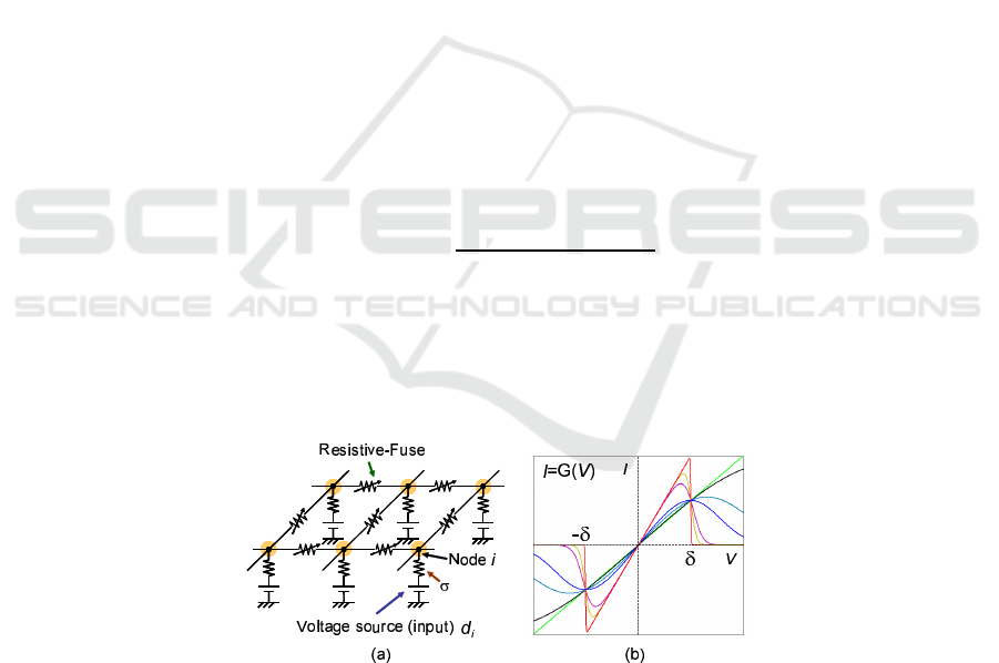
ments, as shown in Fig. 1 (a). Each node corresponds to a pixel state f
i,j
, when the
value of each voltage source represents the image input d
i,j
at pixel (i , j). Each node
and voltage source are connected with a linear resistance, whose conductance is σ. The
adjacent nodes are connected with resistive-fuse elements, whose conductance function
is given by
I = G(V ) =
λV
1 + e xp{η(V
2
− δ
2
)}
, (3)
where λ is the conductance of a resistive-fuse, η is a parameter for changing the con-
ductance function, and δ is the threshold value of the resistive-fuse elements. Equa-
tion (3) is derived by using a deterministic mean field approximation to the MRF model
of piecewise smooth surface interpolation [10], and the parameter η in this equation
corresponds to the inverse of the temperature T for simulated annealing [6].
Fig.1. Original analog resistive-fuse network (a), and I-V characteristics (b) of a resistive-fuse
element.
The energy function of this circuit is given by
44

E(f) = σ
X
i,j
(f
i,j
− d
i,j
)
2
+
X
i,j
X
m,n∈N
Z
V
0
G(v)dv, (4)
where N represents the neighboring nodes of (i, j), and V = f
i,j
− f
m,n
.
When η is close to zero, i.e. temperature T is very high, the conductance is almost
linear, as shown in green color in Fig. 1 (b). In contrast, when η is equal to or larger than
unity, i.e. temperature T is very low, the conductance becomes an ideal resistive-fuse
characteristic, which is similar to the line process function, as shown in red color in
Fig. 1 (b).
As described above, the original RFN model uses a continuation method to avoid
the local minimum problem, by gradually changing the parameter η from near zero to
unity or larger than that. This is based on the assumption that the unique minimum of
the convex energy function is close to the global minimum of the final function shape.
In practice, we calculate the pixel state f by using discrete-time dynamics with an
equation derived from the Kirchhoff’s Current Law (KCL). The dynamics is given by
f
i,j
(t + 1) = f
i,j
(t) − ξ{
X
m,n∈N
G(V ) + 2σ(f
i,j
− d
i,j
)}, (5)
where ξ is a step size parameter of gradient descent. The change of η is called an
annealing process, and the annealing schedule is usually as follows:
η(t + 1) = kη(t), (6)
where t is the index of iterations, and k is a real number which fulfills k ∈ (1, 2] [6,9].
3 Limitations of Original RFN Model
The RFN model mainly has two limitations in actual applications, and each of them is
described in a following subsection.
3.1 Dependence on the Parameters
The original RFN model has four parameters for controlling the energy function: λ, σ,
η and δ. Each of them affects the results of edge detection. λ and σ control the strength
of smoothing, while η and δ control the range of that, i.e. the balance of smoothing and
segmentation. Therefore, it is necessary to make clear the relationships between these
parameters for the control of them.
First of all, let us focus our attention on the relationship between λ and σ. It is
obvious that the value of λ/σ determines the constraint of the input image and the
strength of smoothing. Therefore, the results of edge detection not only depend on the
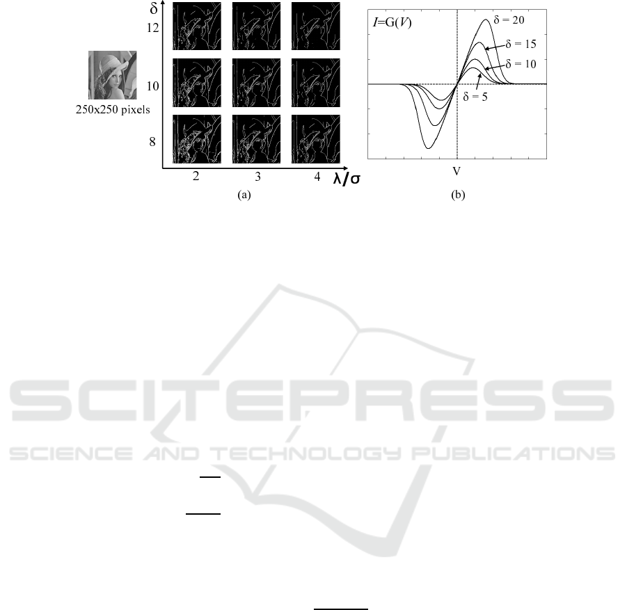
threshold δ, but also sensitively depend on λ/σ, as shown in Fig. 2 (a). The larger the
ratio is, the stronger the strength of smoothing becomes.
Next, we discuss the relationship between η and δ. It is verified from Fig. 2 (b)
that the shapes of the energy function and conductance function G(·) vary according
to both η and δ. This means that the balance of smoothing and segmentation will vary
accordingly when using the same annealing schedule and different δ. This makes it
difficult to select the threshold δ.
45

Fig.2. (a) Edge detection results using RFN model, when η(0) = 0.00055, k = 1.1 and iterations
= 80 in Eq. (6), and (b) Variations of the shape of conductance function, when η = 0.01.
3.2 Complexity of Annealing Process
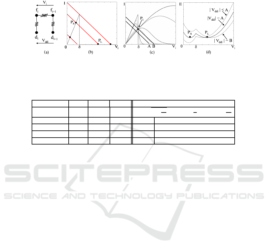
We use a simple circuit as shown in Fig. 3 (a) to discuss the annealing process. In this
case, the energy function is given by
E(f) = σ(f
i
− d
i
)
2
+
Z
V
i
0
G(v)dv + σ(f
i+1
− d
i+1
)
2
+
Z
−V
i
0
G(v)dv, (7)
where V
i
= f
i
− f
i+1
.
When the energy function E(f ) reaches a minimum, we can obtain the following
equations:
∂E
∂f
i
= 2{σ(f
i
− d
i
) + G(V
i
)} = 0. (8)
∂E
∂f
i+1
= 2{σ(f
i+1
− d
i+1
) + G(−V
i
)} = 0. (9)
These two equations mean that E
f
reaches a minimum when the sum of the currents
at each node is zero, i.e. the circuit is in a stable state. Subtracting Eq. (9) from Eq. (8)
gives
G(V
i
) = σ
V
ddi
− V
i
2
, (10)
where V
ddi
= d
i
− d
i+1
. The right-hand side of Eq. (10) is therefore identical to the
current in the linear resistance between f
i
and d
i
. In Fig. 3 (b), the black lines and the
red lines represent I
Ri
(η = 1) and I
ri
, where I
Ri
and I
ri
denote the left-hand and
right-hand side of Eq. (10), respectively. It is clear that I
ri
follows a linear function
of V
i
because V
ddi
is given by the input. Therefore, the intersection points of them
represent the stable states of the circuit.
Figure 3 (b) and Table 1 show that the number of stable states depends on the value
of V
ddi
, which is the intersection point of the red lines and the V
i
-axis. There is only one
46

Fig.3. A simple circuit (a) for discussion, and the relationship (b) between I
i
and V
i
where
V
i
= f
i
− f
i+1
. (c) and (d) show the definitions of A and B using relationship between I
i
and V
i
and that between P
S
and P
L
(η = 1), respectively.
Table 1. Local minimum problem concerned with v.
Value of |V
ddi
| E
min
G U Definitions
|V
ddi
| ∈ (0, δ) single Region S Region S A = δ
q
1 +
2λ
σ
, B = δ(1 +
λ
σ
), C = δ(1 +
2λ
σ
)
|V
ddi
| ∈ (δ, A) multiple Region S Region S G Global E
min
when η ≧ 1
|V
ddi
| ∈ (A, B) multiple Region L Region S U Unique E
min
when η ≈ 0
|V
ddi
| ∈ (B, C) multiple Region L Region L Region S the region where |V
i
| < δ
|V
ddi
| > C single Region L Region L Region L the region where |V
i
| > δ
stable state if V
ddi
is smaller than δ or is large enough. However, there are two stable
states, which are denoted by P
S
and P
L
, if V
ddi
∈ (A, B) where A and B are defined
as shown in Fig. 3 and Table 1.
Note that the series of the conductance function intersect at a point (δ, λδ/2), which
can be calculated from Eq. (3) and is shown as P
I
in Fig. 3 (c). Thus, A, B and C in
Table 1 are defined as follows:
– If V
ddi
= A, E(P
S
) = E(P
L
).
– If V
ddi
= B, the red line moves across P
I
.
– If V
ddi
= C, the red line moves across (δ, λδ).
As described in Sec. 2, the annealing process in RFN model relies on the assumption
that the unique minimum of the convex energy function is close to the global minimum
of the final desired one at each node. Here, “close” can be defined as in the same region
where |V
i
| < δ or |V
i
| > δ, i.e. in the region S or region L.
It is clear from Table 1 that such assumption is not valid when V
ddi
∈ (A, B),
which we called a gray zone. Note that if |V
i
| > δ, the two nodes will be smoothed
from the beginning when using an annealing sequence, such as the annealing schedule
shown in Eq. (6) or a simplified three-stage sequence proposed in [8]. Because there
was no algorithm to prevent the nodes moving into the gray zone, such an annealing
sequence can not always give the global minimum solution at each node, and might
cause over-smoothing and lose some edges. Therefore, the annealing schedule should
be redesigned by considering the relationship between δ, η and λ/σ.
47

4 Improved RFN Model
In order to improve the RFN model, we first introduce self-adjusting functions of λ
and η to reduce the number of parameters to be controlled. Then, we propose a new
annealing sequence for fast and robust edge detection.
4.1 Self-adjusting of λ
We first propose a self-adjusting function of λ as shown in Eq. (11), which has the
similar effect as the annealing process.
λ
m,n
(t + 1) =
(
λ
m,n
(t)(1 + h
λ
), |V | < δ,
λ
m,n
(t)(1 − h
λ
), otherwi se.
(11)
Here, h
λ
is a small positive number and can be determined by the number of iterations
and the range of adjustment.
By using this self-adjusting function of λ, we can set σ and the initial value of λ
as constants, and let λ adjust itself to change the value of λ/σ according to the local
voltage difference. Thus, the manual control of λ and σ becomes unnecessary. Further-
more, this self-adjusting can also improve the robustness of the model because it can
reduce the length of gray zone by decreasing λ/σ when |V | > δ.
4.2 Self-adjusting of η
In order to keep the balance of smoothing and segmentation, we obtain Eq. (12) for the
scaling of conductance function when parameters except η and δ remain identical.
G
1
(V )|
V =kδ
1
: G
2
(V )|
V =kδ
2
= δ
1
: δ
2
, (12)
where k is a certain real number. Thus, we obtain the condition as follows by substitut-
ing Eq. (3) into Eq. (12).
η
1
δ
2
1
= η
2
δ
2
2
(13)
This means that η can be adjusted by δ and the desired shape of the conductance func-
tion.
Summarizing the above, the number of parameters need to be controlled can be
reduced to one, i.e. only the threshold δ, by using the self-adjusting functions of λ and
η. This result significantly simplifies the control of the parameters, and makes it easier
to select the appropriate threshold δ.
4.3 New Annealing Sequence
We propose a heating-and-cooling annealing sequence, and employ a “shaping” pro-
cess, which is named after that in the die making, to reduce the complexity and ambi-
guity of the input image for robust edge detection. The details of the proposed annealing
sequence are as follows. If the defined threshold value is δ
0
,
48

1. “Sharpening” stage: δ = δ
0
/2 and η = 1.
2. “Shaping” stage: δ = δ
0
and η = 1.
3. “Heating” stage: δ = δ
0
and η = 0.1/δ
2
.
4. “Cooling” stage: δ = δ
0
and η = 5/δ
2
.
In the first stage, we use a small δ to sharpen blurred boundaries. During this stage,
the interactions between two nodes where |V | > δ
0
/2 will be cut off and blurred bound-
aries will be sharpened by the smoothing in a small range.
In the second stage, we set δ = δ
0
and η = 1 to calculate the rough results which
obviously include the local minimum and small regions.
In the third stage, we use a small η, i.e. high temperature to smooth small regions
and to lead to global minimum.
In the final stage, we use a large η, i.e. low temperature to “cool” the pixel states
down for coarse edge detection. Note that η is a little smaller than unity in the final
stage. This is because that the binary resistive-fuse characteristic is known as lack of
robustness [11]. Therefore, we use η = 5/δ
2
in the final stage, whose characteristic is
close to that when η = 1, but more convex around where |V | = δ. Therefore, it may
lead to less local minimum in the interactions with neighboring eight nodes.
In summary, we propose a heating-and-cooling annealing sequence, and employ
“sharpening” and “shaping” processes to improve the robustness of the model. Ideal an-
nealing sequences have to smooth noise and small regions at the same time, while keep-
ing the boundaries of large regions. However, simple cooling-down annealing cannot
achieve these functions due to the uncertainty of the input image, and may cause over-
smoothing. In contrast, the proposed annealing sequence can sharpen blurred bound-
aries and reduce noise in the input image before the “heating” stage for smoothing the
small regions. Therefore, the proposed annealing sequence can achieve more robust
detection than simple cooling-down sequences.
5 Simulation Results and Discussion
Figure 4 (a) shows processing results obtained by applying the self-adjusting function
of λ to the original RFN model. It is verified that these results are less sensitive to the
initial value of λ/σ compared with Fig. 2 (a). Figure 4 (b) shows the scaling of the
shape of conductance function, by keeping ηδ
2
constant.
We also evaluated the similarity between the results where (initial value of ) λ/ σ
is two and is four as shown in Table 2. The similarity is defined as the ratio of the
count of identical edge pixels to that of all the edge pixels. In the simulation, 15 images
are selected from 4.1.01 to 4.2.07 in the USC-SIPI Image Database [12]. By comparing
3rd-column with 4th-column in Table 2, it is verified that our self-adjusting function can
significantly weaken the dependence of the model on λ/σ, so that it can increase the
similarities of edge detection results when changing λ/σ. Furthermore, the similarities
of edge detection results come to more than 90% by additionally using our new anneal-
ing sequence as shown in the 5th-column in Table 2. Therefore, the manual control of
λ and σ is unnecessary any more.
Figure 5 shows processing results for images with gradation. The rectangular region
in the input image has a gradation of 10 levels per pixel in 256-level grayscale. These
49

Fig.4. (a) Edge detection results using self-adjusting of λ. The horizontal axis represents the
initial value of λ/σ. (b) Scaling of the shape of conductance function G(·), by using ηδ
2
= 1.
Fig.5. Edge detection results in the case of gradation. Input image (a) with a gradation, and
edge detection results using original RFN model (b), a simplified RFN model (c) in [8] using a
three-stage-cooling annealing sequence, and our proposed RFN model (d).
Table 2. Similarity Evaluation of Edge Detection Results.
δ
Original Adjusting Proposed
model of λ only model
Lena
12 55.09% 69.13% 91.44%
10 58.14% 74.36% 93.32%
8 56.46% 77.59% 93.64%
Average
12 56.65% 69.43% 92.94%
10 57.41% 73.85% 93.61%
8 57.12% 75.67% 94.18%
results show that the original RFN model with an annealing process described in Eq. (6)
can only detect coarse edges, and the model with a simplified three-stage-cooling an-
nealing sequence [8] failed to detect correct edges in the gradation region. In contrast,
the proposed model in this paper can detect coarse edges when δ > 10, and can detect
fine edges when δ ≤ 10.
50

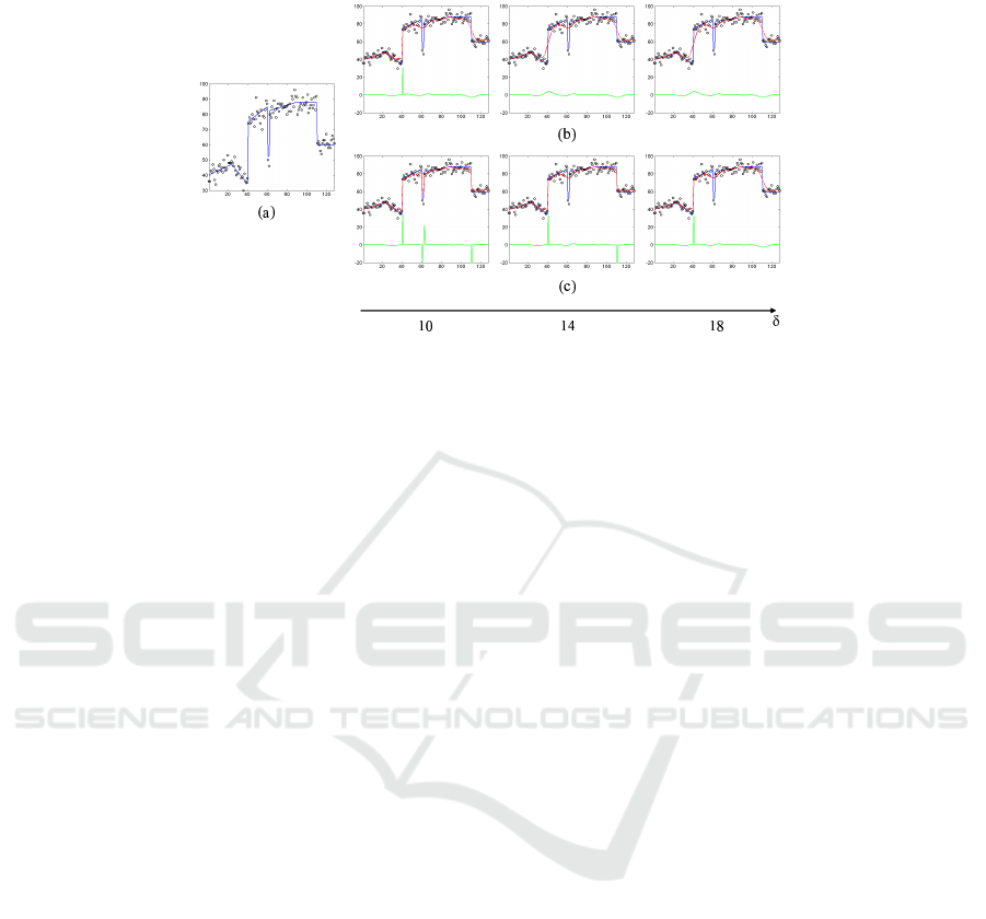
Fig.6. Edge detection results using one-dimension input data with Gaussian white noise. Input
data (a), and edge detection results using original RFN model (b) and proposed model (c). Here,
red color shows the pixel state, and green color shows the first derivation of that.
Figure 6 shows some results using input data shown in black color in Fig. 6 (a),
which is obtained by adding Gaussian white noise (sigma = 4) to the data shown in
blue color. In this simulation, λ/σ in the original RFN model and its initial value in
the proposed model were set to three. It is verified that original RFN model can detect
almost no edges because the boundaries are over-smoothed, as shown in Fig. 6 (b). In
contrast, the proposed model can control the level of edge detection, as shown in Fig. 6
(c), when λ
min
= 2 and λ
max
= 4.
6 Conclusions
We analyzed the resistive-fuse network model for coarse edge detection and clarified
its limitations. First, we proposed self-adjusting functions to simplify the parameter
control. We concluded that only the threshold δ has to be controlled, and the local-
adjusting of λ improves the robustness of edge detection. Then, we proposed a new
annealing sequence for fast and robust detection. It was verified that the proposed model
can detect edges more correctly than the original one, even if an input image includes a
gradation.
Acknowledgements
This work was partly supported by fund from MEXT, Japan, via a Knowledge Cluster
Initiative Second Stage program, granted to Fukuoka Cluster for Advanced System LSI
Technology Development.
51

References
1. Phan, R., Androutsos, D.: Content-based retrieval of logo and trademarks in unconstrained
color image databases using color edge gradient co-occurrence histograms. Computer Vision
and Image Understanding 114 (2010) 66–84
2. Tsai, T. H., Chen, Y. C., Fang, C. L.: 2DVTE: A two-directional videotext extractor for rapid
and elaborate design. Pattern Recognition 42 (2009) 1496–1510
3. Toulminet, G., Bertozzi, M., Mousset, S., Bensrhair, A., Broggi, A.: Vehicle detection by
means of stereo vision-based obstacles features extraction and monocular pattern analysis.
IEEE Trans. on Image Processing 15 (2006) 2364–2375
4. Naito, T., Ito, T., Kaneda, Y.: The obstacle detection method using optical flow estimation at
the edge image. In: IEEE Intelligent Vehicles Symposium, Istanbul, Turkey (2007) 817–822
5. Harris, J. G., Koch, C., Staats, E., Luo, J.: Analog hardware for detecting discontinuities in
early vision. Int. Journal of Computer Vision 4 (1990) 211–223
6. Geman, S., Geman, D.: Stochastic relaxation, Gibbs distributions, and the Bayesian restora-
tion of images. IEEE Trans. on Pattern Analysis and Machine Intelligence 6 (1984) 721–741
7. Kawashima, Y., Atuti, D., Nakada, K., Okada, M., Morie, T.: Coarse image region segmen-
tation using region- and boundary-based coupled MRF models and their PWM VLSI im-
plementation. In: Int. Joint Conf. on Neural Networks (IJCNN2009), Atlanta, USA (2009)
1559–1565
8. Nakano, T., Morie, T., Ishizu, H., Ando, H., Iwata, A.: FPGA implementation of resistive-
fuse networks for coarse image-region segmentation. Intelligent Automation and Soft Com-
puting 12 (2006) 307–316
9. Blake, A.: Comparison of the efficiency of deterministic and stochastic algorithms for visual
reconstruction. IEEE Trans. on Pattern Analysis and Machine Intelligence 11 (1989) 2–12
10. Geiger, D., Girosi, F.: Parallel and deterministic algorithms from MRF’s: Surface recon-
struction. IEEE Trans. on Pattern Analysis and Machine Intelligence 13 (1991) 401–412
11. Harris, J.G.: Analog models for early vision. PhD thesis, California Institute of Technology
(1991)
12. (USC-SIPI) http://sipi.usc.edu/database/.
52
