PREDICTING GROUND-BASED AEROSOL OPTICAL DEPTH
WITH SATELLITE IMAGES VIA GAUSSIAN PROCESSES
Goo Jun, Joydeep Ghosh
Department of Electrical and Computer Engineering, University of Texas, Austin, TX, U.S.A.
Vladan Radosavljevic, Zoran Obradovic
Information Science and Technology Center, Temple University, Philadelphia, PA, U.S.A.
Keywords:
Aerosol, AERONET, MODIS, Gaussian Process, Active Learning, Spatio-temporal Data Mining.
Abstract:
A Gaussian process regression technique is proposed to predict ground-based aerosol optical depth measure-
ments from satellite multispectral images, and to select the most informative ground-based sites by active
learning. Satellite images provide spatial and temporal information in addition to the spectral features, and
such heterogeneity of available features is captured in the Gaussian process model by employing an additive
set of covariance functions. By finding an optimal set of hyperparameters, relevance of each additional in-
formation is automatically determined. Experiments show that the spatio-temporal information contributes
significantly to the regression results. The prediction results are not only more accurate but also more in-
terpretable than existing approaches. For active learning, each spatio-temporal setup is evaluated by an
uncertainty-sampling algorithm. The results show that the active selection process benefits most from the
spatial information.
1 INTRODUCTION
Aerosols are microscopic particles or liquid drops that
are suspended in the Earth’s atmosphere, and have
significant effects on human health (Baron, 2006) and
climate changes (Solomon et al., 2007). Aerosols are
produced by natural and man-made sources and both
reflect and absorb incoming solar radiation. One of
the biggest challenges of current climate research is
to characterize large spatial and temporal variations
of aerosol concentrations, compositions, and sizes,
which requires an integrated approach that effectively
combines various types of measurements and mod-
eling strategies. One way to quantitatively measure
aerosol concentration is estimating the amount of sun-
light absorbed by aerosols, which is called the aerosol
optical depth (AOD) (Dubovik and King, 2000).
There are two major types of instruments whose
measurements can provide info about AOD:
1) Ground instruments, represented by Aerosol
Robotic Network (AERONET) is a global network
of about 250 operational radiometers (Holben et al.,
1998). AERONET provides more accurate measure-
ments with higher temporal resolution compared to
the satellite-based observations, but the data is avail-
able only from a limited number of sites at fixed loca-
tions.
2) Satellite instruments, such as Moderate Resolu-
tion Imaging Spectroradiometer (MODIS).MODIS is
a multispectral sensing instrument in NASA’s Terra
and Aqua satellites (King and Kaufman, 1992). The
MODIS data covers the entire Earth’s surface on
a daily basis, but is usually less accurate than the
ground-based information.
Most operational aerosol prediction algorithms
are deterministic, constructed as inverse operators of
high-dimensional non-linear functions according to
the domain knowledge (Remer et al., 2006). As an
alternative, a novel statistical approach of training a
nonlinear regression model using the satellite obser-
vations as inputs and ground based measurements as
targets was suggested in (Han et al., 2006). It has been
shown that such a statistical approach could improve
the accuracy of predictions significantly as compared
to the operational domain-based methods.
The statistical model proposed in this paper has
two objectives: one is making better and more inter-
pretable AOD retrievals for locations without ground
sensors, and the other is assisting the placements
of ground-based sensors to obtain more informative
groundtruth. The first objective is addressed by adopt-
370
Jun G., Ghosh J., Radosavljevic V. and Obradovic Z..
PREDICTING GROUND-BASED AEROSOL OPTICAL DEPTH WITH SATELLITE IMAGES VIA GAUSSIAN PROCESSES.
DOI: 10.5220/0003115203700375
In Proceedings of the International Conference on Knowledge Discovery and Information Retrieval (KDIR-2010), pages 370-375
ISBN: 978-989-8425-28-7
Copyright
c
 2010 SCITEPRESS (Science and Technology Publications, Lda.)

ing a Gaussian process (GP) regression model that can
easily incorporate auxiliary information such as spa-
tial and temporal information from the satellite mea-
surements. Importances and sensitivities of these fea-
tures are automatically determined by tuning hyper-
parameters of covariance functions. The second is ob-
jective is addressed by employing an active learning
algorithm to select the most informative sites from a
fixed set of candidate locations. Uncertainty scores
for active learning can be easily approximated by the
predictive variances of the fitted Gaussian process. In
this study we are interested in prediction of AODs
although the proposed methods are applicable to a
larger class of remote sensing problems.
2 RELATED WORK
Non-linear regression models in data-driven predic-
tion of atmospheric properties were discussed in
(M
¨
uller et al., 2003). Statistical methods for the
prediction of AOD at a global scale from integrated
ground and satellite-based data were proposed in
(Han et al., 2006), where neural networks trained
on satellite observations spatially-temporally merged
with AERONET measurements were used to predict
AOD. This approach achieved higher prediction accu-
racy than the currently used operational knowledge-
based algorithm (Han et al., 2005), and could aid
domain scientists in understanding sources of cor-
rectable prediction errors (Vucetic et al., 2008).
A neural network-based regression algorithm was
proposed for AOD retrieval by Radosavljevic et al
(Radosavljevic et al., 2009). The authors also con-
sidered a scenario that a number of AERONET sites
are removed from operation, and proposed a method
to maintain the most informative sites. The proposed
goodness criterion for the selection was how close the
accuracy of a regression model built on data from a
reduced sensor set was to the accuracy of a model
built of the entire set of sensors. This approach does
not utilize spatial nor temporal information in regres-
sion, though. An active learning algorithm has been
proposed by Das et al (Das et al., 2009), where an
ensemble of neural networks are constructed by boot-
strapping. In this work, spatial and temporal diversi-
ties are used in the active selection process, but not
included in the prediction model, either.
The proposed method exploits spatio-temporal
correlation between instances using GP regression.
Statistical modeling of spatially varying data has long
been studied as an important field of statistics, called
spatial statistics or geostatistics. Kriging is a well-
known technique to model spatial dependencies of
data, and it has been widely applied to various prob-
lems of spatial statistics (Cressie, 1993). The kriging
approach has recently been adopted by the machine
learning community, where it is referred to as a Gaus-
sian process model (Rasmussen and Williams, 2005).
The next section summarizes the key features of this
model.
3 GAUSSIAN PROCESSES
A jointly Gaussian random vector x =
[x
1
, x
2
, x
3
, ...x
n
]
T
is denoted as x ∼ N (µ, Σ), where
µ is the mean vector and Σ is the covariance matrix.
One useful property of a Gaussian random vector
is that conditional and marginal distributions of
Gaussian random vectors are also Gaussian. A
Gaussian process is a random process such that all
finite dimensional distributions of the process are
jointly Gaussian random vectors (Rasmussen and
Williams, 2005).
Let x be a random process indexed by s, then
x(s) is a Gaussian process if and only if x =
[x(s
1
), x(s
2
), ..., x(s
n
)]
T
is a jointly Gaussian random
vector for any finite set of S = {s
1
, s
2
, ..., s
n
}. As
a Gaussian distribution is defined by its mean and
covariance, a Gaussian process is fully defined by
a mean function µ(s) and a covariance function
k(s
1
, s
2
), and denoted as x(s) ∼ GP(µ(s), k(s
1
, s
2
)).
In Gaussian process regression (GPR), the target vari-
able is modeled by a Gaussian random process. Let
us assume that values of x are observed for some S =
{s
1
, s
2
, ..., s
n
}, and x(s) is modeled as x(s) = f (s)+ε,
where ε is an additive white Gaussian noise term,
ε ∼ N (0, σ
2
ε
). We assume a (zero-mean) Gaussian
process prior for f (s):
f (s) ∼ GP(µ(s) = 0, k(s
1
, s
2
)) .
In regression problems, we are interested in mak-
ing predictions based on the training data x =
[x
1
(s
1
), ..., x
n
(s
n
)]
T
. The predictive distribution of an
out-of-sample instance x
∗
(s
∗
) can be easily derived
from the conditional distribution of jointly Gaus-
sian random vectors, and is also Gaussian: x
∗
(s
∗
) ∼
N (µ
∗
(s
∗
), σ
2
(s
∗
)):
µ
∗
(s
∗
) = k(s
∗
, S)[K
SS
+ σ
2
ε
I]
−1
x ,
σ
2
(s
∗
) = k(s
∗
, s
∗
) + σ
2
ε
− k(s
∗
, S)[K
SS
+ σ
2
ε
I]
−1
k(S, s
∗
) ,
where k(s
∗
, S) = [k(s
∗
, s
1
), k(s
∗
, s
2
), ..., k(s
∗
, s
n
)],
k(S, s
∗
) = k(s
∗
, S)
T
, and K
SS
is a matrix such that its
(i, j)-th element K
i j
= k(s
i
, s
j
). As can be seen in the
formula, the covariance function k(s
1
, s
2
) fully deter-
mines the characteristics of a Gaussian process.
PREDICTING GROUND-BASED AEROSOL OPTICAL DEPTH WITH SATELLITE IMAGES VIA GAUSSIAN
PROCESSES
371

Table 1: List of features from MODIS data.
Feature Description
m
i
Average spectral responses (4-dim)
σ
i
Standard deviations (4-dim)
a
i
Measurement angles (4-dim)
t
i
Temporal information (d
i
, h
i
)
s
i
Longitude and latitude (φ, θ)
4 METHODS
Gaussian process regressions are used to predict the
AERONET AOD values from the spatio-temporally
collocated MODIS data. Table 1 shows the 16 fea-
tures available from the MODIS data.
Since we have heterogeneous features, using a sin-
gle covariance function with the Euclidean distance
measure is not appropriate. Instead, each subset of
features is modeled using a separate covariance func-
tion designed just for the features. First, isometric
squared exponential covariance functions are used for
the baseline features.
k
1
(m
i
, m
j
) = v
2
1
exp −
||m
i
− m
j
||
2
2λ
2
m
!
,
k
2
(a
i
, a
j
) = v
2
2
exp −
||a
i
− a
j
||
2
2λ
2
a
!
.
There are two different features in the temporal in-
formation t
i
= (d
i
, h
i
), where d
i
indicates day of the
year and h
i
is the time of the day in minutes. Since d
i
and h
i
could have different roles in the prediction of
aerosol depths, a non-isometric covariance function is
employed to allow different length scales:
k
3
(t
i
, t
j
) = v
2
3
exp −
∆
d
(d
i
, d
j
)
2
2λ
2
d
−
∆
h
(h
i
, h
j
)
2
2λ
2
h
!
.
Because of the periodic nature of temporal features,
distances ∆
d
and ∆
h
are adjusted for properly inter-
pretation of the actual temporal differences:
In case of spatial information, s
i
= (φ
i
, θ
i
) is a
coordinate in the spherical coordinate system. The
Euclidean distance is not a correct distance measure
for our problem, since we want the geodesic distance
along the surface of the earth. The geodesic dis-
tance on the surface of a sphere is usually referred
to as the great-circle distance. The haversine formula
is used to approximate the angular distance (Sinnott,
1984). The great-circle distance is approximated as
the arc length obtained from the angular distance:
R∆
s
, where R is the radius of the Earth. We do not
consider R as a factor since it will be automatically
incorporated in the length parameter, λ
s
. The co-
variance function for the spatial information is hence
modeled as:
k
4
(s
i
, s
j
) = v
2
4
exp −
∆
s
(s
i
, s
j
)
2
2λ
2
s
!
.
It is also possible to treat longitude and latitude data
separately instead of using the great circle distance,
since the measurements could be more affected from
the longitude information than from the latitudes. We
tried the setup also, but did not get good results. It
also appears that the hyperparameters for longitude
and latitude covariance functions are not much differ-
ent, which means that there is not much advantage in
the separation approach.
The spatial covariance matrix is not positive defi-
nite, because we have multiple instances of data col-
lected from each location. Many s
i
’s have the exactly
same value; hence the resulting covariance matrix has
identical rows and columns. Since a positive definite
covariance matrix is required for GPR, we add small
perturbations to the values of s
i
, proportional to the
measurement noise. In Table 1, σ
i
is a feature that in-
dicates the standard deviations in the measured spec-
trum. We used the averaged standard deviation,
¯
σ
i
, to
add random noise to the spatial features:
φ
i
= φ
i
+ N(0,
¯
σ
i
) , θ
i
= θ
i
+ N(0,
¯
σ
i
) .
The overall covariance function is obtained by
simply adding the aforementioned covariance func-
tions, as a sum of positive definite kernels is also
a positive definite kernel (Rasmussen and Williams,
2005). We consider four different settings in this pa-
per. k
ε
= v
2
ε
δ
i j
is a term for noise, where δ
i j
is a
kronecker-delta function:
1. Baseline: k = k
1
+ k
2
+ k
ε
.
2. Temporal: k = k
1
+ k
2
+ k
3
+ k
ε
.
3. Spatial: k = k
1
+ k
2
+ k
4
+ k
ε
.
4. Spatio-temporal: k = k
1
+ k
2
+ k
3
+ k
4
+ k
ε
.
Once the covariance function is designed, the next
step is selecting the hyperparameters. The most com-
plicated model is the spatio-temporal model, which
has ten hyperparameters. Hyperparemeters are se-
lected by minimizing the negative log likelihood by
the gradient descent method. To avoid local min-
ima and for faster search, a randomized algorithm is
used by selecting a random subset of samples from the
training data. Each randomized search result is then
evaluated using the entire training data, and the set of
hyperparameters with the highest log-likelihood score
is selected.
An uncertainty sampling approach (Lewis and
Gale, 1994) is used to perform active learning. In con-
trast to loss-reduction methods, uncertainty sampling
generally does not require the model to be re-trained
for every unlabeled instance. Instead, each instance in
the unlabeled dataset is assigned an uncertainty score
predicted by the model trained on the labeled data.
In the Gaussian process model, there is a natural mea-
sure of uncertainty, the posterior variance σ
2
(s
∗
). The
KDIR 2010 - International Conference on Knowledge Discovery and Information Retrieval
372

predictive distribution of the model provides the vari-
ance of an out-of sample instance as well as the mean.
At each stage of the active learning process, we sim-
ply select the site that has the highest average vari-
ance.
5 EXPERIMENTS
GP Regression. Datasets for experiments were
created by collecting spatio-temporally MODIS and
AERONET measurement data over 70 AERONET
sites for years 2005 and 2006. The 2005 data is sub-
sampled to construct 10 randomly selected training
sets, where each set contains data from 30 AERONET
sites. We used the same set of training datasets as
used in (Radosavljevic et al., 2009) to make the results
comparable; hence please refer to the paper for details
on the data preparation. Baseline, temporal, spatial,
and spatio-temporal GP models are trained with each
training set, and tested on the test data from 2006.
In previous studies, it was observed that the variance
of the AERONET AOD data increases as the AOD
value increases, and using square-root values of the
target variable helps making better predictions. We
use the same approach, and R
2
scores are calculated
by first squaring the predicted values and comparing
them to the original AOD values. 10 sets of 300 ran-
domly selected samples are used for hyperparameter
optimization.
Table 2 shows the R
2
scores obtained from the four
proposed settings, as well as the current state-of-the-
art approach using an ensemble of neural nets (Ra-
dosavljevic et al., 2009). The spatio-temporal model
shows better results than the baseline results in a sta-
tistically significant manner, and the spatial informa-
tion appears to be more informative than the temporal
information. Table 3 shows the estimated hyperpa-
rameters (v
2
1
, . . . v
2
4
, v
2
ε
) that determine how much each
covariance function contributes to the predicted value.
Hyperparameters are estimated using one of the train-
ing datasets. As shown in the table, the spectral fea-
tures are the most dominant features, and the mea-
surement angles second. The spatial information has
smaller significance, but is much more relevant than
the temporal information. Table 4 shows the esti-
mated length parameters (λ
m
, λ
a
, λ
d
, λ
t
, λ
s
) using the
same training set, indicating that the degree of cor-
relation associated with each feature. Since different
features have different physical dimensions, units of
each length scale are shown in the table. It is notice-
able that the time of the day has very short length pa-
rameter, λ
t
, meaning that the prediction depends on
the time features only if the time difference between
Table 2: R
2
scores with baseline, temporal, spatial, and
spatio-temporal features, and using neural networks.
Basel. Temporal Spatial Spatio-temp. NN*
Mean 0.7160 0.7376 0.7622 0.7726 0.746
Median 0.7208 0.7401 0.7706 0.7748 0.754
Std. Dev. 0.0162 0.0243 0.0263 0.0180 0.042
*(Radosavljevic et al., 2009)
Table 3: Variance parameter associated with each covari-
ance function.
Baseline Temporal Spatial Spatio-temp.
v
2
1
(spectral) 1.560 2.8123 1.1548 1.528
v
2
2
(angle) 0.5471 1.6525 0.6615 0.8122
v
2
3
(temporal) - 0.00450 - 0.00190
v
2
4
(spatial) - - 0.00876 0.0112
v
2
ε
(noise) - 0.00638 0.00613 0.00718
the test and the training instances is very small.
Active Learning. For active learning experiments,
five sites are randomly selected to construct the initial
training data. One site is added to the training data
after each active learning step. Each site in 2005 data
has 70 instances, and the uncertainty score for each
site is the average over all 70 instances. Each exper-
imented is repeated 10 times. To save computational
time, five sets of 200 randomly selected samples are
used to optimize hyperparameters. Using fewer sam-
ples resulted in slightly lower R
2
scores for the same
number of randomly selected sites compared to the
results in the previous section.
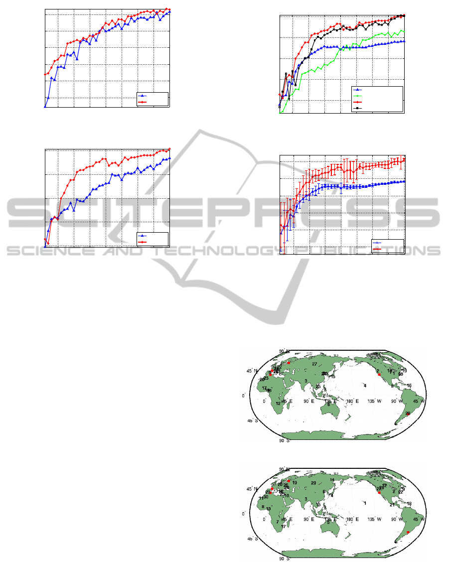
Fig. 1 shows the learning curves from temporal
and spatial methods, and each method is tested us-
ing passive (random) and active learning algorithms.
The spatial results show significant improvements by
using active learning algorithms, but not the tempo-
ral results. A plausible explanation is that the use of
the temporal kernel yields high variances on the in-
stances having longer temporal distances, but having
temporally distant measurements in 2005 do not guar-
antee the same informational gain for the 2006 data.
In contrast, spatial distances remain the same both in
the training and the test data. Fig. 2(a) shows the ac-
tive learning results for four GP setups. It is clear that
temporal information adds valuable information for
Table 4: Length parameter associated with each covariance
function.
Baseline Temporal Spatial Spatio-temp.
λ
m
(normalized) 0.2136 0.3031 0.1704 0.3441
λ
a
(degree) 86.91 105.4 101.2 121.7
λ
d
(days) - 17.23 - 14.75
λ
t
(minutes) - 0.2958 - 0.1267
λ
s
(radian) - - 0.1348 0.1491
PREDICTING GROUND-BASED AEROSOL OPTICAL DEPTH WITH SATELLITE IMAGES VIA GAUSSIAN
PROCESSES
373

5 10 15 20 25 30 35 40
0.5
0.55
0.6
0.65
0.7
0.75
Number of sites added
R
2
Temporal
Random
Active
(a) Temporal
5 10 15 20 25 30 35 40
0.6
0.65
0.7
0.75
0.8
Number of sites added
R
2
Spatial
Random
Active
(b) Spatial
Figure 1: R
2
scores from passive and active learning algo-
rithms with different features.
making predictions, but not for active learning, com-
pared to the spatial information. The best (spatial)
and the worst (baseline) learning curves with error
bars of one standard deviation are presented in Fig.
2(b) to show statistical significance of results. Fig.
3 shows the locations of 30 actively selected sites on
the world maps. All experiments are started with the
same initial training set, marked with red squares. 30
actively selected sites are shown with numbers that in-
dicates the order of selection. It is observable that the
baseline result has regions with densely located sites,
while the spatial one has more dispersed selections.
6 CONCLUSIONS
Gaussian process regressions are used to predict
ground-based aerosol optical depth measurements
with satellite-taken multispectral images. Heteroge-
neous features with spatial and temporal information
are incorporated together by employing a set of co-
variance functions, and it is shown that the spatio-
temporal information adds valuable information to the
regression model. An uncertainty-sampling based ac-
tive learning algorithm is tested with each regression
setup. It turns out that the active selection process
5 10 15 20 25 30 35 40
0.6
0.65
0.7
0.75
0.8
Number of sites added
R
2
Active Learning Results
Baseline
Temporal
Spatial
Spatio−temporal
(a) Active learning results
5 10 15 20 25 30 35 40
0.55
0.6
0.65
0.7
0.75
0.8
Number of sites added
R
2
Active Learning Results
Baseline
Spatial
(b) Baseline vs. spatial
Figure 2: Active learning results. (a) results from four dif-
ferent settings. Error bars are removed for visibility (b) spa-
tial active learning compared to the base line with error bars
of one standard deviation.
(a) Baseline
(b) Spatial
Figure 3: Sites picked by active learning with four different
settings. Red squares are five sites included in the initial
training set, and numbers indicate the order of selection by
active learning.
KDIR 2010 - International Conference on Knowledge Discovery and Information Retrieval
374

benefits most by adding spatial information compared
to the baseline method. As a possible extension to
the proposed method, the square-root transform of the
dependent variable can be incorporated into the Gaus-
sian process model, but this idea requires further stud-
ies since it involves designing a non-stationary covari-
ance function.
ACKNOWLEDGEMENTS
This work was supported by NSF Grants IIS-0705815
and IIS-0612149.
REFERENCES
Baron, P. (2006). Generation and Behavior of Air-
borne Particles (Aerosols). National Institute of
Occupational Health and Safety, http://www. cdc.
gov/niosh/topics/aerosols/pdfs/Aerosol 101. pdf. Re-
trieved on June.
Cressie, N. (1993). Statistics for Spatial Data. Wiley, New
York.
Das, D., Obradovic, Z., and Vucetic, S. (2009). Active
selection of sensor sites in remote sensing applica-
tions. In IEEE International Conference on Data Min-
ing (ICDM 09).
Dubovik, O. and King, M. (2000). A flexible inversion al-
gorithm for retrieval of aerosol optical properties from
Sun and sky radiance measurements. Journal of Geo-
physical Research, 105(D16):20676.
Han, B., Obradovic, Z., Li, Z., and Vucetic, S. (2006).
Data Mining Support for the Improvement of MODIS
Aerosol Retrievals. In IEEE International Conference
on Geoscience and Remote Sensing Symposium, 2006.
IGARSS 2006, pages 2453–2456.
Han, B., Vucetic, S., Braverman, A., and Obradovic, Z.
(2005). Construction of a geospatial predictor by fu-
sion of global and local models. In Proccedings of
8th International Conference on Information Fusion.
Citeseer.
Holben, B., Eck, T., Slutsker, I., Tanre, D., Buis, J., Setzer,
A., Vermote, E., Reagan, J., Kaufman, Y., Nakajima,
T., et al. (1998). AERONET–A federated instrument
network and data archive for aerosol characterization.
Remote Sensing of Environment, 66(1):1–16.
Kaufman, Y., Tanr
´
e, D., Remer, L., Vermote, E., Chu, A.,
and Holben, B. (1997). Operational remote sensing
of tropospheric aerosol over land from EOS moder-
ate resolution imaging spectroradiometer. J. Geophys.
Res, 102(17):051–17.
King, M. and Kaufman, J. (1992). Remote sensing of cloud,
aerosol, and water vapor properties from the Moderate
Resolution Imaging Spectrometer (MODIS). IEEE
Transactions on Geoscience and Remote Sensing,
30(1).
Lewis, D. D. and Gale, W. A. (1994). A sequential algo-
rithm for training text classifiers. In Proceedings of the
17th Annual International ACM SIGIR Conference on
Research and Development in Information Retrieval,
pages 3–12. Springer-Verlag New York, Inc.
M
¨
uller, M., Kaifel, A., Weber, M., Tellmann, S., Burrows,
J., and Loyola, D. (2003). Ozone profile retrieval
from Global Ozone Monitoring Experiment (GOME)
data using a neural network approach (neural network
ozone retrieval system (NNORSY)). J. Geophys. Res,
108(D16):4497.
NASA (retrieved in 2010). Official MODIS website,
http://modis.gsfc.nasa.gov/.
Radosavljevic, V., Vucetic, S., and Obradovic, Z. (2009).
Reduction of ground-based sensor sites for spatio-
temporal analysis of aerosols. In SensorKDD ’09:
Proceedings of the Third International Workshop on
Knowledge Discovery from Sensor Data, pages 71–
78, New York, NY, USA. ACM.
Rasmussen, C. (1996). Evaluation of Gaussian processes
and other methods for non-linear regression. PhD the-
sis, University of Toronto.
Rasmussen, C. E. and Williams, C. K. I. (2005). Gaussian
Processes for Machine Learning. The MIT Press.
Remer, L., Tanr
´
e, D., Kaufman, Y., Levy, R., and Mattoo, S.
(2006). Algorithm for remote sensing of tropospheric
aerosol from MODIS: Collection 005. modis. gsfc.
nasa. gov/data/atbd/atbd mod02. pdf.
Seung, H. S., Opper, M., and Sompolinsky, H. (1992).
Query by committee. In Proceedings of the Fifth An-
nual Workshop on Computational Learning Theory,
pages 287–294, Pittsburgh, PA, USA. ACM Press.
Sinnott, R. (1984). Virtues of the Haversine. Sky and tele-
scope, 68:158.
Solomon, S., Qin, D., Manning, M., Chen, Z., Marquis, M.,
Averyt, K., Tignor, M., and Miller, H. (2007). IPCC
2007. Climate Change 2007: the Physical Science Ba-
sis Contribution of Working Group I to the Fourth
Assessment Report of the Intergovernmental Panel on
Climate Change.
Vucetic, S., Han, B., Mi, W., Li, Z., and Obradovic, Z.
(2008). A Data-Mining Approach for the Validation
of Aerosol Retrievals. IEEE Geoscience and Remote
Sensing Letters, 5(1):113–117.
PREDICTING GROUND-BASED AEROSOL OPTICAL DEPTH WITH SATELLITE IMAGES VIA GAUSSIAN
PROCESSES
375