MODELLING A BACKGROUND FOR BACKGROUND

SUBTRACTION FROM A SEQUENCE OF IMAGES

Formulation of Probability Distribution of Pixel Positions

Suil Son, Young-Woon Cha and Suk I. Yoo

School of Computer Science and Engineering, Seoul National University, 599 Gwanak-ro, Seoul, Korea

Keywords: Background subtraction, Foreground detection, Probability distribution of pixel positions, Intensity clusters,

Kernel density estimation.

Abstract: This paper presents a new background subtraction approach to identifying the various changes of objects in

a sequence of images. A background is modelled as the probability distribution of pixel positions given

intensity clusters, which is constructed from a given sequence of images. Each pixel position in a new image

is then identified with either a background or a foreground, depending on its value from probability

distribution of pixel positions representing a background. The presented approach is illustrated using two

examples. As compared to traditional intensity-based approaches, this approach is shown to be robust to

dynamic textures and various changes of illumination.

1 INTRODUCTION

Detecting a meaningful foreground from a sequence

of images, known as background subtraction, has

been studied intensively due to its wide area of

application such as tracking, identification and

surveillance. Two issues in developing background

subtraction methods are how to resolve the change

of illumination due to noise or light and how to

manage dynamic textures such as swaying tree or

flow of water.

To manage the change of illumination, most of

background subtraction methods have used intensity

distributions (Wren, Darrelll and Pentland, 1997,

Stauffer and Grimson, 1999, Elgammal, Harwood,

and Davis, 2000, Power and Schoonees, 2002,

Zivkovic and Heijden, 2006, Dalley, Migdal, and

Grimson, 2008). Using intensity distributions,

however, does not work very well when there is the

large change of illumination in all pixels on the

image. To resolve dynamic textures, a mixture of

Gaussian (Stauffer and Grimson, 1999, Power and

Schoonees, 2002, Zivkovic and Heijden, 2006,

Dalley et al, 2008) and the kernel density estimation

(Elgammal et al, 2000, Mittal and Paragios, 2004)

have been suggested. To recognize the background

having small motion correctly, spatial information of

objects is necessary. A window formed with

neighbours of a pixel may be used to reflect such

spatial information (Elgammal et al, 2000, Dalley et

al, 2008). Although the approach using windows

reduces false detection of foreground for dynamic

textures, it is not easy to define the exact size of a

window in advance. Sheikh and Shah (2005)

suggested joint distribution of positions and

intensities to reflect the spatial information. Since

this joint representation of image pixels reflects the

local spatial structure, it works well on motion of

background objects. However, it has a difficulty

with the curse of dimensionality from its high

dimensional data representation.

This paper presents a new approach to relaxing

those difficulties of the traditional background

subtraction methods: A background is modelled as

the probability distribution of pixel positions given

intensity clusters. An image in a given sequence is

assumed to have M intensity sources. From the

image having M intensity sources, M intesity

clusters can be formulated. Although it is not easy to

figure out the optimal number of M from a given

image, specially when the image is complex with

various objects, the value of M is assumed to be not

larger than six in general due to the range of grey

level from 0 to 255.

For each of the M intensity clusters, the distribu-

tion of pixel positions is then computed from the

sequence of images. The computed distribution of

545

Son S., Cha Y. and Yoo S..

MODELLING A BACKGROUND FOR BACKGROUND SUBTRACTION FROM A SEQUENCE OF IMAGES - Formulation of Probability Distribution of

Pixel Positions.

DOI: 10.5220/0003141105450551

In Proceedings of the 3rd International Conference on Agents and Artiﬁcial Intelligence (ICAART-2011), pages 545-551

ISBN: 978-989-8425-40-9

 2011 SCITEPRESS (Science and Technology Publications, Lda.)

pixel positions, however, suffers from the disconti-

nuity between pixels due to the limited number of

images in the sequence. By smoothing this disconti-

nuity using kernel density estimation, the probability

distribution of pixel positions modelling a back-

ground is finally constructed. Each pixel position in

the new image is then identified with either a

foreground or a background, depending on its value

from the probability distribution constructed.

In the following section related previous works

are visited. In section 3, generation of a probability

distribution of pixel positions given intensity

clusters from a sequence of images is described. The

process to identify each pixel position in a new

image with either a background or a foreground is

explained in section 4. Finally the presented

approach is illustrated and compared to the intensity-

based approach in section 5.

2 RELATED WORKS

Most of traditional background subtraction models

estimate intensity distributions for each pixel

position (Paccardi, 2004).

Stauffer and Grimson (1999) have modelled the

value of each pixel as a mixture of M Gaussian

distributions in order to represent intensity variations

caused by small motion of objects in the background

like swaying trees or flow of water. The probability

that a pixel position x has an intensity x

at time t is

estimated as

()()

()

(2 ) | |

tj jtj







 











(1)

where w

is the weight for each Gaussian distribution,

is the mean and Σ

=σ

I is the covariance of the jth

Gaussian distribution, and M is the number of

Gaussians. The M is selected from 3 to 5. This

model assumes that the intensity value may result

from some candidate sources each of which is

modelled as a Gaussian. Therefore, an intensity

value has several distributions where it may come

from. This model can adapt to small change of

intensity or shape in background but in the case

where the background has slightly large variations, it

fails to achieve correct identification.

Dalley et al. (2008) have proposed a model

modified from the Stauffer and Grimson(1999)’s

one. In this model, a set of mixture components that

lie at the local spatial neighbourhood of a pixel are

suggested rather a mixture that lies at the same pixel.

The probability that a pixel position i has an

intensity c

is estimated as

()

() (| , )

j Neighbour

iijj

P wNcc











(2)

where μ

is the mean, Σ

is the covariance of

Gaussian distribution N at a pixel position j, and w

is a mixture weight of a neighbour j. This model

considers intensity distributions at neighbours of a

pixel simultaneously. Therefore, intensity variations

caused by small motion of objects in background

can be correctly identified with a background.

However, the background subtraction result of this

model is dependent on the size of a window applied

to include neighbours but the optimal window size is

hardly obtained.

Elgammal et al (2000) suggested the kernel

density estimation to model intensity distribution

with multimodality. When there are n samples of

intensities, the true distribution of these intensities

may be dense where the samples are closely located

and may be sparse where the samples are scattered.

These characteristics are modelled as a sum of many

kernels centred at each sample. Since this model is a

data driven approach, the multimodality of

distribution for these data is naturally reflected

without any assumption of the number of modes.

This model for intensity distribution of a pixel can

be represented as follows

() ( )K

tti



 



(3)

where x

and x

are intensities of a pixel x at time t

and i ,respectively, n is the number of samples, and

K is a kernel function. The Gaussian function is

usually used for the kernel function K. This model

can handle situations where the background of

scenes contains small motion but it still suffers from

large motion and illumination changes. To overcome

this difficulty, this model proposed additional policy

considering the displacement probability P

Neighbour

()

() max ( | )

Neighbour

y Neighbour x

ytt

PPBxx





(4)

where B

is a background sample for a pixel y. This

approach significantly reduced false detection of a

background but it still has a difficulty in selecting

optimal neighbours.

All approaches discussed above are same in

considering distribution of intensities for a given

pixel position. In this framework, motion of objects

in background was modelled as variations of

intensities and neighbours of a pixel are introduced

ICAART 2011 - 3rd International Conference on Agents and Artificial Intelligence

546

to reflect more spatial variations. These approaches

may be regarded as an indirect approach to handle

spatial variations. In this paper, we model spatial

variations directly using distribution of pixel

positions given intensity values.

3 MODELLING A BACKGROUND

In this section we first describe how to generate M

intensity clusters from a given image and then

construct from a sequence of images the probability

distribution of pixel positions for each of M intensity

clusters modelling a background.

3.1 Generation of M Intensity Clusters

When a given image has M intensity sources with

background, it is assumed that the image can be

characterized with M different intensity clusters. The

k-means algorithm (Bishop, 2006) is then used to

generate the M intensity clusters:

Let μ

be a mean of intensity values of those

pixels forming the i

th cluster C

where i=1, …, M.

and let I

be an intensity value of a pixel at location

(x,y) of the image I with height of H and width of W.

The k-means algorithm defines the membership

value r

xyi

of the intensity value I

with respect to the

cluster C

where x=1,2,…,W and y=1,2,…,H, to be

1, argmin| |

xyi

if i I

otherwise

















(5)

where j=1,2,…,M.

The value of μ

is initially set to a small value

and the r

xyi

is computed by (5). With the computed

value of r

xyi

, the μ

is then updated by (6). This

process is repeated until there is no change in the

values of μ

and r

xyi

. The value of r

xyi

indicates

whether or not the pixel at (x,y) is associated with

the cluster C

yi xy









(6)

For example, the image with two objects,

rectangle and circle, is characterized with three

intensity clusters as shown in Fig. 1.

(a) (b)

Figure 1: Three intensity clusters, (b), (c), and (d), shown

as white areas, from a given image of (a).

3.2 Probability Distribution of Pixel

Positions for Intensity Clusters

When M intensity clusters are generated from one

image, the same number of clusters can be generated

from each of images in a sequence. Once we obtain

the same number of clusters from all images in the

sequence, we can count the number of occurrence of

each pixel position with respect to each of the M

clusters. The occurrence of pixel positions for a

given cluster may then represent statistical data for

the intensity value associated with that cluster.

Let

be the lth image, l=1,2,…,N, from a

sequence of N images. The histogram h

(x,y;C

defined to be the number of times from the N images

that each position (x,y) is located in the cluster C

, is

then

( , ; ) | { : 1, 1, 2,..., } |

N xyi

hxyC lr l N

(7)

where

is the value of

in the lth image

Since each pixel considered as a background in a

new image has its intensity value similar to those of

the associated pixels in all of the N images in a

sequence, its h value becomes large for one of M

clusters. Each pixel considered as a foreground,

however, has its intensity value different from those

of the associated pixels in all the N images so that its

h value becomes small for the associated cluster. A

foreground comes from an unusual event and objects

formed with those pixels considered as foregrounds

may be observed in a few of the N images.

MODELLING A BACKGROUND FOR BACKGROUND SUBTRACTION FROM A SEQUENCE OF IMAGES -

Formulation of Probability Distribution of Pixel Positions

547

(a)

(b-1) (b-2)

(c-1)

(c-2)

(d-1)

(d-2)

Figure 2: Histograms and Probability distributions of

positions for each intensity cluster constructed from for a

sequence of 30 images of (a): (b-1) h

(x,y;C

), (b-2)

P(x,y|C

), (c-1) h

(x,y;C

), (c-2) P(x,y|C

), (d-1) h

(x,y;C

and (d-2) P(x,y|C

Since the histogram reflects the direct result from

a given sequence of images, it suffers from its

discontinuity for small motion of objects due to the

limited number of images in the sequence. To

overcome such difficulty, the kernel density estima-

tion is suggested to smooth the discontinuity.

The kernel density estimation (KDE) is one of

well-known nonparametric density estimation

methods (Elgammal et al, 2000, Bishop 2006). The

KDE has many kernels centred at each data point so

as to construct a probability distribution of the data.

The KDE has the property to relax discontinuity of

data and make smooth change between data. Thus

we propose a kernel density estimation weighted by

the histogram to obtain the smooth and continuous

distribution of pixel positions.

When there is a histogram h

(x,y;C

) of an

intensity cluster C

, the position distribution for the

cluster C

, P(x,y|C

), is given by the following kernel

density estimation.

(, | )

(, ) ( , )

(, )

;

qpi q p

qpi

Pxy C

hxy xxy y

hxy





 



(8)

where K is a two dimensional kernel function. The

Gaussian kernel is usually used for the kernel

function as follows:







(,) exp

uv u v



K

(9)

where b is a bandwidth of the kernel function.

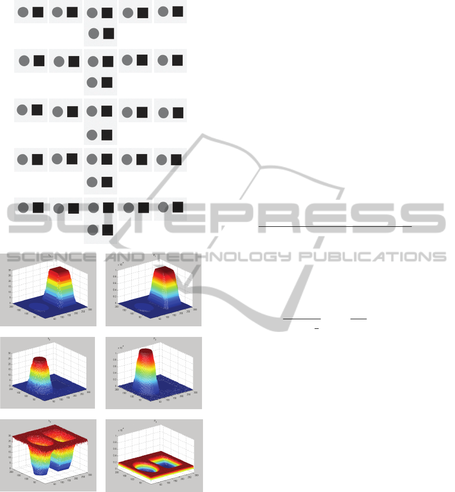
As one example, suppose that a sequence of 30

images shown in Fig. 2 (a) is given where each

image has three intensity sources. Three intensity

clusters can then be generated. For each of three

intensity clusters, the histogram and the associated

probability distribution of pixel positions are

computed as shown in Fig. 2 (b-1), (b-2), (c-1), (c-2),

(d-1), and (d-2). As compared to each of histograms,

the associated probability distribution is smoother

and normalized.

4 DETECTING A FOREGROUND

Once the pixel position distribution for each of

intensity clusters is constructed, the identification of

each pixel position in a new image as a background

or a foreground is achieved by labelling it as

follows:

Let the new image be I

N+1

. The



, the cluster

membership value for I

N+1

, is computed using the

k-means algorithm described in section 2. Each pixel

ICAART 2011 - 3rd International Conference on Agents and Artificial Intelligence

548

position (x,y) on the I

N+1

is then labelled with L(x,y)

defined to be



(, ) (, | )

Txyi

Lxy f Pxy C r









(10)

(a) (b)

Figure 3: (a) A given new image and (b) a detected

foreground shown as a white area.

where f

is a threshold function given by

()

if z T

otherwise











(11)

with a predefined value T.

Suppose that a given pixel position (x,y) on the

new image I

N+1

is one of them forming the jth

intensity cluster. Then the value of



becomes 1

only when i=j. If its value from

P(x,y|C

) is less than

T, then it is detected as a foreground. Otherwise, it is

a background.

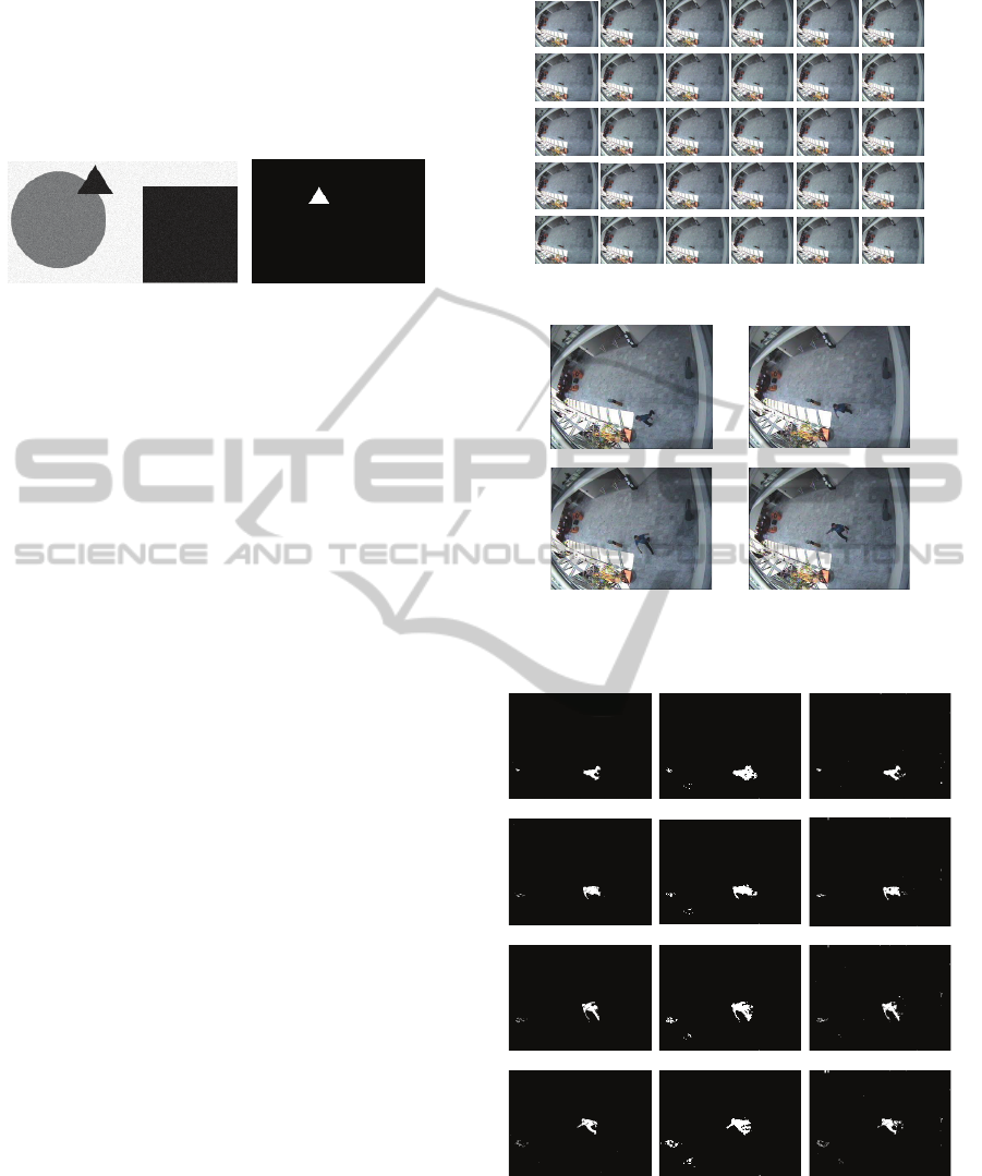
For example, given a sequence of thirty images

in Fig. 2 (a), if a new image in Fig. 3 (a) is given,

those pixels forming triangle shown in Fig. 3 (b) are

detected as a foreground.

5 EXAMPLES

Our approach is illustrated using two examples

having dynamic textures and large change of

illumination, respectively. It is also compared to the

intensity-based approach using KDE (IBA-KDE)

(Elgammal et al, 2000) and to the intensity-based

approach using Gaussian Mixture Model (IBA-

GMM) (Dalley et al, 2008).

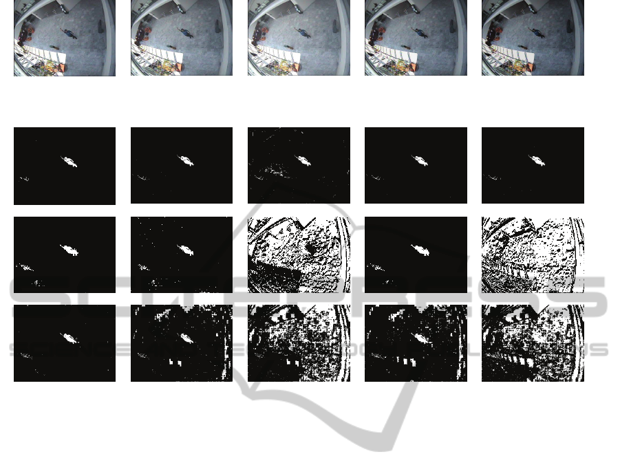
As the first example having dynamic textures, a

sequence of 30 images shown in Fig. 4 and four new

images shown in Fig. 5 are assumed. From each

image in the sequence where four intensity sources

are assumed, four intensity clusters are generated.

For each of the four intensity clusters, the proba-

bility distribution of pixel positions is then computed

from 30 images in the sequence.

Figure 4: A sequence of 30 images.

(a)

(b)

(c)

(d)

Figure 5: Four new images with different shapes of a

walking man.

(a-1)

(a-2)

(a-3)

(b-1)

(b-2)

(b-3)

(c-1)

(c-2)

(c-3)

(d-1)

(d-2)

(d-3)

Figure 6: Results from images in Fig. 5 by ours, IBA-KDE,

and IBA-GMM.

From the first new image in Fig. 5(a), the result by

our approach is shown in Fig. 6(a-1), the result by

the IBA-KDE is in Fig. 6(a-2), and the result by the

MODELLING A BACKGROUND FOR BACKGROUND SUBTRACTION FROM A SEQUENCE OF IMAGES -

Formulation of Probability Distribution of Pixel Positions

549

(a)

(b)

(c)

(d)

(e)

Figure 7: Five new images with different illumination.

(a-1)

(b-1)

(c-1)

(d-1)

(e-1)

(a-2)

(b-2)

(c-2)

(d-2)

(e-2)

(a-3)

(b-3)

(c-3)

(d-3)

(e-3)

Figure 8: Results from images in Fig. 7 by ours, IBA-KDE, and IBA-GMM.

IBA-GMM is in Fig. 6(a-3). Similarly, from the next

three new images in Fig. 5(b), 5(c), 5(d), the result

by ours is in Fig. 6(b-1), 6(c-1), 6(d-1), the result by

the IBA-KDE in Fig. 6(b-2), 6(c-2), 6(d-2), and the

result by the IBA-GMM in Fig. 6(b-3), 6(c-3), 6(d-

3). As noticed by comparing three results in Fig. 6,

our approach detected the foreground successfully

but the IBA-KDE and the IBA-GMM did not.

As the second example having large change of

illumination, a sequence of 30 images in Fig. 4 and

five new images in Fig. 7 are assumed. All of the

five new images represent the same scene with

different illumination where the image in (a) is an

original image and others in (b), (c), (d), and (e) are

modified in their intensities with +10, +30, -10, and

-30, respectively. The same probability distribution

of pixel positions computed in the first example is

then used for detecting a foreground from the five

new images.

From Fig. 7(a), the result by ours is in Fig. 8(a-1),

the result by the IBA-KDE is in Fig. 8(a-2), and the

result by the IBA-GMM is in Fig. 8(a-3). Similarly,

from Fig. 7(b), 7(c), 7(d), 7(e), the result by ours is

in Fig. 8(b-1), 8(c-1), 8(d-1), 8(e-1), the result by

IBA-KDE in Fig. 8(b-2), 8(c-2), 8(d-2), and the

result by the IBA-GMM in Fig. 8(b-3), 8(c-3), 8(d-

3), 8(e-3). As shown in Fig. 8, our approach detected

a foreground successfully from four of the five

images except (c) with a little false detection.

However, both of the IBA-KDE and the IBA-GMM

failed to detect a foreground from each of (c) and (e).

Further the IBA-GMM results in false detection

from both of (b) and (d).

From these two examples, our approach is shown

to be robust to dynamic textures and also large

change of illumination as compared to the IBA-KDE

and the IBA-GMM.

Finally, the results from using five different

values of threshold with four different numbers of

clusters are shown in Fig. 9 where as the number of

clusters gets larger, the smaller value of threshold

becomes more appropriate. Note however that the

number of clusters is closely related to the number

of intensity sources in the given image.

6 CONCLUSIONS

For modelling a background from a sequence of

images, we presented the probability distribution of

pixel positions for intensity clusters. To detect a

foreground from a given new image, probability of

each pixel position is obtained from the probability

ICAART 2011 - 3rd International Conference on Agents and Artificial Intelligence

550

M=3

M=4

M=5

M=6

T=0.00000025 T=0.0000005 T=0.000001 T=0.000002 T=0.000004

Figure 9: Results from an image in Fig. 7-(a) using different values of threshold with different numbers of clusters.

distribution. If it is less than some predefined

threshold, it is detected as a foreground. Otherwise,

it is a background. Our approach is illustrated to be

not to suffer from dynamic textures and large change

of illumination, as compared to the intensity-based

approaches. Finally the work to find the general

formula to find the optimal number of intensity

sources from a given image is left as the future work.

ACKNOWLEDGEMENTS

The ICT at Seoul National University provides

research facilities for this study.

REFERENCES

Bishop, C. M., 2006, Pattern recognition and machine

learning, Springer, 1

edition.

Dalley, G., Migdal, J., and Grimson, W. E. L., 2008,

Background subtraction for temporally irregular

dynamic textures, IEEE Workshop on Applications of

Computer Vision.

Elgammal, A., Harwood, D., and Davis L., 2000, Non-

parametric model for background subtraction,

European Conference on Computer Vision.

Mittal, A., and Paragios, N., 2004, Motion-based

background subtraction using adaptive kernel density

estimation, IEEE Computer Vision and Pattern

Recognition.

Piccardi, M., 2004, Background subtraction techniques: a

review, IEEE International Conference on Systems,

Man and Cybernetics.

Power, P. W., and Schoonees, J. A., 2002, Understanding

background mixture models for foreground

segmentation, Proceedings Image and Vision

Computing New Zealand.

Sheikh, Y., and Shah, M., 2005, Bayesian modelling of

dynamic scenes for objects detection, IEEE

Transaction on Pattern Analysis and Machine

Intelligence.

Stauffer, C., Grimson, W. E. L., 1999, Adaptive

background mixture models for real-time tracking,

IEEE Computer Vision and Pattern Recognition.

Wren, C., Azarbayejani, A. Darrel, T., and Pentland, A. P.,

1997, Pfinder: real-time tracking of the human body,

IEEE Transaction on Pattern Analysis and Machine

Intelligence.

Zivkovic, Z., and Heijden, F. V. D., 2006, Efficient

adaptive density estimation per image pixel for the

task of background subtraction, Pattern Recognition

Letters.

MODELLING A BACKGROUND FOR BACKGROUND SUBTRACTION FROM A SEQUENCE OF IMAGES -

Formulation of Probability Distribution of Pixel Positions

551