GRAPH BASED SOLUTION FOR SEGMENTATION TASKS IN CASE

OF OUT-OF-FOCUS, NOISY AND CORRUPTED IMAGES

Anita Keszler, Tam

as Szir

anyi

Distributed Events Analysis Group, Computer and Automation Research Institute

Hungarian Academy of Sciences, Budapest, Hungary

Zsolt Tuza

Combinatorial Computer Science Research Group, Computer and Automation Research Institute

Hungarian Academy of Sciences, Budapest, Hungary

Keywords:

Image segmentation, Focus map, Graph-based clustering, Dense subgraph mining.

Abstract:

We introduce a new method for image segmentation tasks by using dense subgraph mining algorithms. The

main advantage of the present solution is to treat the out-of-focus, noise and corruption problems in one uniﬁed

framework, by introducing a theoretically new image segmentation method based on graph manipulation.

This demonstrated development is however a proof of concept: how dense subgraph mining algorithms can

contribute to general segmentation problems.

1 INTRODUCTION

We introduce a new method for image segmentation

tasks by using dense subgraph mining algorithms.

Image classiﬁcation based on the automatically ex-

tracted location of the main objects for indexing and

retrieval purposes is a still active research area on the

different levels of machine vision. We contribute to

this problem an automatic method ﬁnding image ar-

eas out of focus.

The goal in the segmentation is a binary task: dis-

criminate the focused and out of focus areas. The

method ﬁrst builds up a graph, where pixels are the

vertices and edges are weighted by the interpixel simi-

larities in a given radius. In image segmentation graph

cut and spectral analysis methods (Kim and Hong,

2009)(Shi and Malik, 2000)(Cousty et al., 2009) are

the most frequently used solutions, however these

methods usually have several drawbacks. The main

disadvantage in this type of application is the ﬁxed

number of segments these methods give as an output,

where this number is often independent of the intput

dataset. However, in case of dense subgraph mining

algoritmhs there are numerous approaches where we

can avoid this problems, although applied for social

interaction mining (Du et al., 2007),(Faloutsos et al.,

2004)(Mishra et al., 2007).

2 FINDING THE AREA OF

FOCUS

This development is however a proof of concept: how

dense subgraph mining algorithms can contribute to

general image segmentation problems. The present

problem, segmenting focused areas was an unsolved

one until (Kovacs and Sziranyi, 2007). That paper

suggested a solution using localized blind deconvo-

lution, without any a priori knowledge about the im-

age or the shooting conditions and using a new er-

ror measure for area classiﬁcation. Previous meth-

ods (Lim et al., 2005) used edges or autocorrelation

methods to ﬁnd sharp areas, but their efﬁciency was

weaker for the real focus detection than that of (Ko-

vacs and Sziranyi, 2007). The focus-map detection

methods are usually based on the assumption that pix-

els are smoothed in out-of-focus areas resulting in

lower contrast there. While edge based methods con-

sider the local derivatives to measure smoothness, the

blind deconvolution based method (Kovacs and Szi-

ranyi, 2007) makes estimation on the local image con-

tent itself. The previous methods do not handle the

case when the in-focus condition is evaluated against

noisy and corrupted (e.g. scratched or badly transmit-

ted) images.

100

Keszler A., Szirányi T. and Tuza Z..

GRAPH BASED SOLUTION FOR SEGMENTATION TASKS IN CASE OF OUT-OF-FOCUS, NOISY AND CORRUPTED IMAGES.

DOI: 10.5220/0003379401000105

In Proceedings of the International Conference on Imaging Theory and Applications and International Conference on Information Visualization Theory

and Applications (IMAGAPP-2011), pages 100-105

ISBN: 978-989-8425-46-1

 2011 SCITEPRESS (Science and Technology Publications, Lda.)

(a) Original image. (b) The area of focus.

Figure 1: Test results on images with blurred background.

The present method is also based on the fact that lo-

cal contrast is weaker in blurred areas, but noise and

data corruption is considered on a graph theoretical

view-point. However, this procedure is different from

conventional morphology or correlation based image

corrections, like ones in (Licsar et al., 2010). The

main advantage of the present solution is to treat the

out-of-focus, noise and corruption problems in one

uniﬁed framework, by introducing a theoretically new

image segmentation method based on graph manipu-

lation.

2.1 Finding the Blurred Area in an

Image

The method of blurred area detection is to identify

the clusters of pixels corresponding to the blurred ar-

eas. The ﬁrst phase of ﬁnding the clusters is to detect

the cluster cores (corresponding pixels), then the next

step is to classify the remaining pixels (blurred or fo-

cused area) depending on their similarities to cluster

cores. If a pixel is similar to any of the found cores, it

will belong to a blurred area in the image.

The mining of the cluster cores is an essential part

of numerous dense subgraph mining algorithms. A

core is a set of vertices that is sufﬁciently dense com-

pared to the average density of the graph. Especially

in a large graph it is a hard task to ﬁnd a fast way of

recognizing the cores. In (Mishra et al., 2003) the

authors present a theoretical approach to solve this

problem for bipartite graphs in O(|V |) time, mining

ε-bicliques. |V | denotes the number of objects to be

clustered. Although the running time is linear in the

number of nodes, it is exponential in the parameter

showing how close we are to the complete bipartite

subgraphs. Another disadvantage is that it is only ap-

plicable if the size of a cluster is also O(|V |), and as it

is based on random sampling, it only ﬁnds the clusters

with a given probability.

In our solution, the running time of the core ﬁnd-

ing FINDCORES() algorithm is O(|V |

) for an arbi-

trary graph. However, it is suitable for any cluster

size, and ﬁnds all cluster cores parallelly. Besides

this, if the input graph is sparse (E = O(V )), the run-

ning time is O(V ). Since in case of graphs of images,

where only the neighboring pixels are connected, we

have a sparse graph, we get a linear running time in

the number of pixels. We work with a modiﬁed mini-

mum weight spanning tree algorithm, and we use the

Kruskal-algorithm as a basis.

Since we do not need to have a subgraph without

circles, we only use the idea that the order of con-

necting vertices depends on how similar they are. An

obvious problem is to deﬁne the stopping conditions

of the algorithm. We will use d

limit

as a threshold to

ensure that in each cluster core the nodes are similar

enough. In each step, when the Kruskal-algorithm de-

cides whether an edge should be a part of the spanning

tree, we also check the diameter of the evolving com-

ponent. Let P be the pixel set of the image, and let M

be the feature matrix, where each µ

row is the corre-

sponding feature vector of pixel v

∈ V . The steps of

the algorithm are the following:

Algorithm [ClusterCores]=FINDCORES(M,

limit

1. Compute the distance between feature vectors

2. Increasing order of the distance values:

Dist

order

3. Inicialization: Let G = (V,E) be a graph,

′

={}; i = 1;

4. x = Dist

order

(i);

5. if x < d

limit

E = E ∪x; i = i + 1; else discard x;

6. If there are edges left, go to step 4.

7. ClusterCores = Connected components

The focused areas of the images are more de-

tailed than the blurred ones, hence differences be-

tween neighboring pixels tend to be higher. On the

other hand the components we get as an output (Clus-

terCores) contain the pixel-sets with the smallest dif-

ferences. These pixel-sets correspond to the blurred

areas of the image. Since we only need to make a dif-

ference between focused and blurred parts, as it was

mentioned before, the pixels corresponding to any of

the ClusterCores, will belong to the blurred area. The

limit

is the maximum weight of the edges we choose

GRAPH BASED SOLUTION FOR SEGMENTATION TASKS IN CASE OF OUT-OF-FOCUS, NOISY AND

CORRUPTED IMAGES

101

(a) (b) (c) (d) (e)

Figure 2: (a) Original image. (b) MSE-based method. (c) PSF-based algorithm. (d) Localized blind deconvolution algorithm.

(e) The presented method.

for the cluster cores and is set based on the distribu-

tion of edges. The algorithm will stop when adding

the edges corresponding to weight of d

limit

results in

the smallest changes in the output.

2.2 Test Results

We present two results for the FINDCORES() algo-

rithm for detecting blurred regions on several images

on Fig. 1: (a), (c) show the original images. The

pixels of the ClusterCores were masked and the re-

maining ones are selected as focused area, presented

on (b) and (d).

We have compared our results to other methods,

see Fig. 2. Fig. (a) shows the original image, (b) is

an MSE distance-based extraction algorithm (Kovacs

and Sziranyi, 2005), (c) PSF-based method, while

(d) is the method presented in (Kovacs and Sziranyi,

2007). Compared to the focus map the other algo-

rithms present (b)(c)(d), one should notice that the

proposed algorithms (e) detects the area in focus and

gives an output with a higher (pixel-level) resolution

with a small running time.

3 FINDING THE AREA OF

FOCUS IN A NOISY IMAGE

Handling noisy input data is an important task in fo-

cus detection as well. The proposed method can also

be applied as a preprocessing step for image restora-

tion algorithms, since selecting the area of focus in

noisy images offers the opportunity of applying dif-

ferent deblurring methods for areas of different con-

trast levels. Fig. 3 (a) and (b) present an example

of the original and noisy images. If we use the RGB

codes of the neighboring pixels as feature vectors, the

output of the FINDCORES() algorithm will become

almost unusable (Fig. 3 (c)). Since the algorithm

works on pixel-level, noisy pixel features might re-

sult in high edgeweights, or on the contrary we might

connect pixels that should be separated in the clean

image. To overcome this problem we extend the fea-

ture vectors of the vertices with the features of the

neighboring pixels (8-connection). With this, we get a

more robust method in case of pixel-level noises (Fig.

3 (c)).

4 FINDING THE AREA OF

FOCUS IN CASE OF

PARTIALLY MISSING

INFORMATION

Several problems occur for videos in online transmis-

sion when some portion of the image is missing (lines

or blocks). Since we do not have the data needed to

calculate the distance of these damaged pixels with

the former methods, we need a different model to

make use of the available information.

The role of the graph in the former section was

to ﬁnd the cluster cores corresponding to the blurred

areas in the image. We will use a bipartite graph to

model and cluster the pixels of the cluster cores and

the pixels with damaged feature vectors. An impor-

tant improvement of this structure is applying a bi-

partite graph model complemented with a standard

model, leading to a new way of handling missing

data. The idea is to cluster the damaged feature vec-

tors and the corresponding pixels based on the avail-

able information by ﬁnding the dense bipartite sub-

graphs they belong to. The cores of these dense bi-

partite subgraphs are the cluster cores of the FIND-

CORES(algorithm). The proposed method has the

following steps:

Algorithm [MV]=CLUSTER(M

comp

, M

dam

, ε)

1. [ClusterCores] =FINDCORES(M

comp

limit

)

2. [C

ClCore

] =CALC-

CORECHAR(ClusterCores,ε)

3. [MV

matrix

] =COMPUTE-MV(M

comp

dam

)

IMAGAPP 2011 - International Conference on Imaging Theory and Applications

102

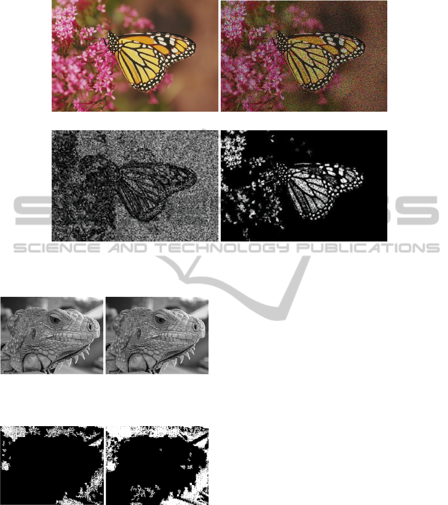
(a) Original image. (b) Noisy image with random noise of 30%.

the algorithm.

(d) Output of the neighborhood-based version

of the algorithm.

Figure 3: Result of the focus-detection in a noisy image using different versions of the algorithm.

(a) (b)

Figure 4: (a) Original test image. (b) Noisy image with

missing pixels of 10%.

Figure 5: Inner steps of the core ﬁnding algorithm. The

white areas present the most strongly connected pixels in

the image.

The FINDCORES() subalgorithm is applied to

detect the cluster cores, based on the pixels with

complete feature vectors (M

comp

). The CALC-

CORECHAR() method calculates a characteristic

vector for each cluster core, using the feature vec-

tors to select the relevant cluster-dependent features.

The pixel feature vectors are compared to the gained

characteristic vectors by the COMPUTE-MV() subal-

gorithm, which gives the membership values of each

pixel concerning each cluster as an output. This func-

tion calculates the membership values for pixel with

complete (M

comp

) and incomplete or damaged (M

dam

)

feature vectors as well.

4.1 Calculating Characteristics using a

Bipartite Graph

In the bipartite graph, the gained ClusterCores of

the FINDCORES() subalgorithm form dense bipartite

subgraphs, where the density deﬁnition is the same as

in (Mishra et al., 2003): Let G = (A,B, E) a bipartite

graph and 0 ≤ ε ≤ 1. A G

′

= (A

′

) subgraph is

an ε-quasi-biclique, if

∀v

∈ A

′

,|N

′

)

′

| ≥ (1 − ε) · |B

′

|,whereN

′

) ∈ B

′

The ε parameter can be bounded from below us-

ing the d

limit

parameter from the FINDCORES() sub-

algorithm. Although these cores are dense compared

to the average density of the graph, if ε ≥ ε

desired

then

to get better results the most weekly connected nodes

should be removed. As a result we get the relevant

features for each cluster core, see Fig. 6.

Based on the feature vectors of the nodes in each

core, we get the cluster characteristics. A weight vec-

GRAPH BASED SOLUTION FOR SEGMENTATION TASKS IN CASE OF OUT-OF-FOCUS, NOISY AND

CORRUPTED IMAGES

103

Figure 6: Cluster cores of the standard graph (left) found by the FINDCORES() method. Bipartite graph model: we determine

the relevant features for each cluster core; Pixels with incomplete feature vectors will be clustered based on the similarities

between their non-missing features and the relevant feature sets of the clusters.

tor is calculated as an average of the feature vectors

in each cluster core and the disparity vector as well.

If the disparity is low, the feature is relevant for the

given cluster. The feature relevance is important also

among the cluster cores. If the disparity within the

clusters is low for a given feature, then it is not suit-

able to make a distinction between the clusters.

The cluster characteristics consist of a characteris-

tics value, derived from the two disparity values, and a

weight value. The steps of the CALC-CORECHAR()

algorithm for calculating the characteristics are as fol-

lows: (The f () function is for normalizing the char-

acteristics.)

In this case, it is an apparent overcomplication to

select relevant features, since now we work with low

dimensional feature vectors. However, the presented

test results were only an illustration of the capacities

of the algorithm. The algorithm is capable of handling

high dimensional feature vectors, for example if the

SIFT features of the pixels are used.

Algorithm [c

ClCore

] = CALC-

CORECHAR (ClusterCores).

1. For each core c

in ClusterCores

2. w

ClCore

(i,k) = avg(µ

) if v

∈ c

3. σ

(i,k) = disp(µ

)

4. For each feature F

ClCores

(k) =

disp(w

ClCore

(i,k))

5. For each core c

in ClusterCores c

ClCore

(i,k) =

f (σ

ClCores

(k)/σ

(i,k))

4.2 Clustering the Nodes

By clustering one usually means deciding to which

cluster core the given node belongs to. Here to each

object we calculate a membership-value, how strong

the connection to each core is, and a conﬁdence value,

representing the reliability of this strenght value.

Algorithm [MV

matrix

]=COMPUTE-MV (M

comp

dam

, c

ClCore

, w

ClCore

1. For each v

in M

comp

and M

dam

2. For each c

cluster core if m

i j

̸= 0

3. di f f (i, j) = abs(m(i) − w

ClCore

( j))

4. d(i) = norm(di f f (i))

5. MV (i, j,k) = d(i) · c

ClCore

( j)

6. MembValue(i, j) = sum

[MV (i, j, k)]

7. Con f idence(i, j) = sum(m

i j

)/F if m

i j

̸= 0

We compare the m(i) feature vector of each vertex

with the cluster weight vector w

ClCore

( j), and we

apply normalization (step 4). The previously calcu-

lated characteristics will be used as relevance measure

weights. The membership values are derived from the

non-missing elements of the feature vectors. The con-

ﬁdence value represents the ratio of the available in-

formation.

Let us notice that every node is re-clustered, even

the ones, we used for ﬁnding the cluster cores. If more

membership values are high in case of a given node,

it means the node belongs to both clusters. This way

the algorithm can be used even if the dataset contains

overlapping clusters.

Figure 7: The foreground part of the image selected by the

algorithm.

IMAGAPP 2011 - International Conference on Imaging Theory and Applications

104

5 CONCLUSIONS

We have implemented a theoretically new image seg-

mentation algorithm, based on graph core mining in

the structure of bipartite graphs. This approach makes

it possible to involve image reconstruction-like oper-

ations into the same framework: focus-detection, de-

noising and patching. This paper is only a posing of

a greater framework, where the method will be devel-

oped by: multi-level clusters, multi-scale evaluation,

texture-analysis and semantic level evaluation. The

above results encourage us to exploit the potential of

graph clustering in more complex image understand-

ing tasks. The algorithm can also be applied as a pre-

processing step for image restoration methods.

REFERENCES

Cousty, J., Bertrand, G., Najman, L., and Couprie, M.

(2009). Watershed cuts: Minimum spanning forests

and the drop of water principle. IEEE Transactions on

Pattern Analysis and Machine Intelligence, 31:1362–

1374.

Du, N., Wu, B., Pei, X., Wang, B., and Xu, L. (2007). Com-

munity detection in large-scale social networks. In

Proceedings of the 9th WebKDD and 1st SNA-KDD

2007 workshop on Web mining and social network

analysis, pages 16–25, New York, NY, USA. ACM.

Faloutsos, C., McCurley, K. S., and Tomkins, A. (2004).

Connection subgraphs in social networks. In Proceed-

ings of the Workshop on Link Analysis, Counterter-

rorism, and Privacy (in conj. with SIAM International

Conference on Data Mining).

Kim, J.-S. and Hong, K.-S. (2009). Color-texture segmenta-

tion using unsupervised graph cuts. Pattern Recogn.,

42(5):735–750.

Kovacs, L. and Sziranyi, T. (2005). Relative focus map es-

timation using blind deconvolution. Optics Letters,

30:3021–3023.

Kovacs, L. and Sziranyi, T. (2007). Focus area extraction

by blind deconvolution for deﬁning regions of interest.

IEEE Transactions on Pattern Analysis and Machine

Intelligence, 29(6):1080–1085.

Licsar, A., Sziranyi, T., and Czuni, L. (2010). Trainable

blotch detection on high resolution archive ﬁlms min-

imizing the human interaction. Machine Vision and

Applications, 21(5):767–777.

Lim, S. H., Yen, J., and Wu, P. (2005). Detection of out-

of-focus digital photographs. Technical Report HPL

2005-14.

Mishra, N., Ron, D., and Swaminathan, R. (2003). On ﬁnd-

ing large conjunctive clusters. In In Computational

Learning Theory, volume 2777, pages 448–462.

Mishra, N., Schreiber, R., Stanton, I., and Tarjan, R. E.

(2007). Clustering social networks. In WAW’07: Pro-

ceedings of the 5th international conference on Algo-

rithms and models for the web-graph, pages 56–67,

Berlin, Heidelberg. Springer-Verlag.

Shi, J. and Malik, J. (2000). Normalized cuts and image

segmentation. IEEE Trans. Pattern Anal. Mach. In-

tell., 22(8):888–905.

GRAPH BASED SOLUTION FOR SEGMENTATION TASKS IN CASE OF OUT-OF-FOCUS, NOISY AND

CORRUPTED IMAGES

105