HIDDEN ATTRACTOR IN CHUA’S CIRCUITS
N. V. Kuznetsov
1,2
, O. A. Kuznetsova
1
, G. A. Leonov
2
and V. I. Vagaytsev
1
1
University of Jyv¨askyl¨a, P.O. Box 35 (Agora), FIN-40014, Jyv¨askyl¨a, Finland
2
Saint-Petersburg State University, Universitetski pr. 28, 198504, Saint-Petersburg, Russia
Keywords:
Chaotic communication, Chua’s circuits, Hidden attractor localization, Hidden oscillation, Harmonic lin-
earization, Describing function method.
Abstract:
Notion of hidden attractor (basin does not contain neighborhoods of equilibria) is discussed. Effective
analytical-numerical procedure for hidden attractors localization is considered. Existence of hidden attrac-
tor in Chua’s circuits is demonstrated.
1 INTRODUCTION
The classical attractors of Lorenz (Lorenz, 1963),
Rossler (Rossler, 1976), Chua (Chua & Lin, 1990),
Chen (Chen & Ueta, 1999), and other widely-known
attractors are those excited from unstable equilibria.
From computational point of view this allows one to
use numerical method, in which after transient pro-
cess a trajectory, started from a point of unstable man-
ifold in the neighborhood of equilibrium, reaches an
attractor and identifies it.
However there are attractors of another type: hid-
den attractors, a basin of attraction of which does not
contain neighborhoods of equilibria (Leonov et. al.,
2011). Here equilibria are not “connected” with at-
tractor and creation of numerical procedure of inte-
gration of trajectories for the passage from equilib-
rium to periodic solution is impossible because the
neighbourhoodof equilibrium does not belong to such
attractor. The simplest examples of systems with such
hidden attractors are hidden oscillations in counterex-
amples to widely-known Aizerman’s and Kalman’s
conjectures on absolute stability (see, e.g., (Leonov,
2010; Leonov et. al., 2010b)). Similar computational
problems arise in investigation of semi-stable and
nested limit cycles in 16th Hilbert problem (see, e.g.,
(Kuznetsov & Leonov, 2008; Leonov & Kuznetsov,
2010; Leonov et. al., 2011)).
Here a special analytical-numerical algorithm for
localization of hidden attractors is considered. Ex-
ample of hidden attractor localization in Chua’s cir-
cuit, which is used for hidden chaotic communication
(Zhiguo et al., 2008), is demonstrated.
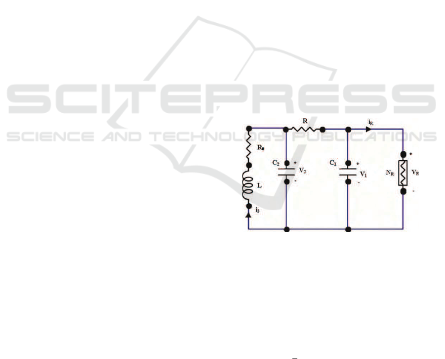
Chua’s circuit (see Fig. 1) can be described by dif-
Figure 1: Classical Chu’s circuit.
ferential equations in dimensionless coordinates:
˙x = α(y− x) − α f(x),
˙y = x− y + z,
˙z = − (βy+ γz).
(1)
Here the function
f(x) = m
1
x+ (m
0
− m
1
)sat(x) =
= m
1
x+
1
2
(m
0
− m
1
)(|x+ 1| − |x− 1|)
(2)
characterizes a nonlinear element, of the system,
called Chua’s diode; α,β,γ,m
0
,m
1
are parameters of
the system. In this system it was discovered the
strange attractors (Chua, 1992; Chua, 1995) called
then Chua’s attractors. All known classical Chua’s at-
tractors are the attractors that are excited from unsta-
ble equilibria. and this makes it possible to compute
such attractors with relative easy (see, e.g., attractors
gallery in (Bilotta & Pantano, 2008).
The applied in this work algorithm shows the pos-
sibility of existence of hidden attractor in system (1).
Note that L. Chua himself, analyzing in the work
279
V. Kuznetsov N., A. Kuznetsova O., A. Leonov G. and I. Vagaytsev V..
HIDDEN ATTRACTOR IN CHUA’S CIRCUITS.
DOI: 10.5220/0003530702790283
In Proceedings of the 8th International Conference on Informatics in Control, Automation and Robotics (ICINCO-2011), pages 279-283
ISBN: 978-989-8425-74-4
Copyright
c
 2011 SCITEPRESS (Science and Technology Publications, Lda.)

(Chua & Lin, 1990) different cases of attractor ex-
istence in Chua’s circuit, does not admit the existence
of such hidden attractor.
2 ANALYTICAL-NUMERICAL
FOR ATTRACTORS
LOCALIZATION
Consider a system
dx
dt
= Px+ ψ(x),x ∈ R
n
, (3)
where P is a constant n× n-matrix, ψ(x) is a continu-
ous vector-function, and ψ(0) = 0.
Define a matrix K in such a way that the matrix
P
0
= P+ K (4)
has a pair of purely imaginary eigenvalues ±iω
0
(ω
0
> 0) and the rest of its eigenvalues have nega-
tive real parts. We assume that such K exists. Rewrite
system (3) as
dx
dt
= P
0
x+ ϕ(x), (5)
where ϕ(x) = ψ(x) − Kx.
Introduce a finite sequence of functions
ϕ
0
(x),ϕ
1
(x),...,ϕ
m
(x) such that the graphs of
neighboring functions ϕ
j
(x) and ϕ
j+1
(x) slightly dif-
fer from one another, the function ϕ
0
(x) is small, and
ϕ
m
(x) = ϕ(x). Using a smallness of function ϕ
0
(x),
we can apply and mathematically strictly justify
(Leonov, 2009; Leonov, 2009; Leonov, 2010; Leonov
et. al., 2010a; Leonov et. al., 2010b) the method of
harmonic linearization (describing function method)
for the system
dx
dt
= P
0
x+ ϕ
0
(x), (6)
and determine a stable nontrivial periodic solution
x
0
(t). For the localization of attractor of original sys-
tem (5), we shall follow numerically the transforma-
tion of this periodic solution (a starting oscillating at-
tractor — an attractor, not including equilibria, de-
noted further by A
0
) with increasing j. Here two cases
are possible: all the points of A
0
are in an attraction
domain of attractor A
1
, being an oscillating attractor
of the system
dx
dt
= P
0
x+ ϕ
j
(x) (7)
with j = 1, or in the change from system (6) to sys-
tem (7) with j = 1 it is observed a loss of stability
bifurcation and the vanishing of A
0
. In the first case
the solution x
1
(t) can be determined numerically by
starting a trajectory of system (7) with j = 1 from the
initial point x
0
(0). If in the process of computation
the solution x
1
(t) has not fallen to an equilibrium and
it is not increased indefinitely (here a sufficientlylarge
computationalinterval[0, T] should always be consid-
ered), then this solution reaches an attractor A
1
. Then
it is possible to proceed to system (7) with j = 2 and
to perform a similar procedure of computation of A
2
,
by starting a trajectory of system (7) with j = 2 from
the initial point x
1
(T) and computing the trajectory
x
2
(t).
Proceeding this procedure and sequentially in-
creasing j and computing x
j
(t) (being a trajectory of
system (7) with initial data x
j−1
(T)) we either arrive
at the computation of A
m
(being an attractor of system
(7) with j = m, i.e. original system (5)), either, at a
certain step, observe a loss of stability bifurcation and
the vanishing of attractor.
To determine the initial data x
0
(0) of starting peri-
odic solution, system (6) with nonlinearity ϕ
0
(x) can
be transformed by linear nonsingular transformation
S to the form
˙x
1
= −ω
0
x
2
+ εϕ
1
(x
1
,x
2
,x
3
),
˙x
2
= ω
0
x
1
+ εϕ
2
(x
1
,x
2
,x
3
),
˙
x
3
= A
3
x
3
+ εϕ
3
(x
1
,x
2
,x
3
)
(8)
Here A
3
is a constant (n − 2) × (n − 2) matrix, all
eigenvalues of which have negative real parts, ϕ
3
is an
(n − 2)-dimensional vector-function, ϕ
1
,ϕ
2
are cer-
tain scalar functions. Without loss of generality, it
may be assumed that for the matrix A
3
there exists
positive number α > 0 such that
x
∗
3
(A
3
+ A
3
∗
)x
3
≤ −2α|x
3
|
2
, ∀x
3
∈ R
n−2
(9)
Introduce the following describing function
Φ(a) =
2π/ω
0
R
0

ϕ
1
((cosω
0
t)a, (sinω
0
t)a, 0)cosω
0
t+
+ϕ
2
((cosω
0
t)a, (sinω
0
t)a, 0)sinω
0
t

dt.
Theorem 1. (Leonov et. al., 2010b) If it can be found
a positive a
0
such that
Φ(a
0
) = 0, (10)
then there is a periodic solution in system (6) with the
initial data x
0
(0) = S(y
1
(0),y
2
(0),y
3
(0))
∗
y
1
(0) = a
0
+ O(ε), y
2
(0) = 0, y
3
(0) = O
n−2
(ε).
(11)
Here O
n−2
(ε) is an (n − 2)-dimensional vector such
that all its components are O(ε).
ICINCO 2011 - 8th International Conference on Informatics in Control, Automation and Robotics
280

3 LOCALIZATION OF HIDDEN
ATTRACTOR IN CHUA’S
SYSTEM
We now apply the above algorithm to analysis of
Chua’s system with scalar nonlinearity. For this pur-
pose, rewrite Chua’s system (1) in the form (3)
dx
dt
= Px+ qψ(r
∗
x), x ∈ R
3
. (12)
Here
P,q,r =




−α(m
1
+ 1) α 0
1 −1 1
0 −β −γ




,


−α
0
0


,


1
0
0


,
ψ(σ) = (m
0
− m
1
)sat(σ).
Introduce the coefficient k and small parameter ε,
and represent system (12) as (6)
dx
dt
= P
0
x+ qεϕ(r
∗
x), (13)
where
P
0
= P+ kqr
∗
=


−α(m
1
+ 1+ k) α 0
1 −1 1
0 −β −γ


,
λ
P
0
1,2
= ±iω
0
, λ
P
0
3
= −d,
ϕ(σ) = ψ(σ) − kσ = (m
0
− m
1
)sat(σ) − kσ.
In practice, to determine k and ω
0
it is used the trans-
fer function W(p) of system (3):
W
P
(p) = r
∗
(P− pI)
−1
q,
where p is a complex variable. Then ImW(iω
0
) =
0 and k is computed then by formula k =
−(ReW(iω
0
))
−1
.
By nonsingular linear transformation x = Sy sys-
tem (13) can be reduced to the form
dy
dt
= Ay + bεϕ(c
∗
y), (14)
where
A,b,c =


0 −ω
0
0
ω
0
0 0
0 0 −d


,


b
1
b
2
1


,


1
0
−h


.
The transfer function W
A
(p) of system (14) can be
represented as
W
A
(p) = W
P
(p).
Further, using the equality of transfer functions of
systems (13) and (14), we obtain
W
A
(p) = r
∗
(P
0
− pI)
−1
q.
This implies the following relations
k =
−α(m
1
+ m
1
γ+ γ) + ω
2
0
− γ− β
α(1+ γ)
,
d =
α+ ω
2
0
− β + 1+ γ+ γ
2
1+ γ
,
h =
α(γ+ β− (1+ γ)d+ d
2
)
ω
2
0
+ d
2
,
b
1
=
α(γ+ β− ω
2
0
− (1+ γ)d)
ω
2
0
+ d
2
,
b
2
=
α

(1+ γ− d)ω
2
0
+ (γ+ β)d

ω
0
(ω
2
0
+ d
2
)
.
(15)
System (13) can be reduced to the form (14) by
the nonsingular linear transformation x = Sy. Having
solved the following matrix equations
A = S
−1
P
0
S, b = S
−1
q, c
∗
= r
∗
S, (16)
one can obtain the transformation matrix
S =


s
11
s
12
s
13
s
21
s
22
s
23
s
31
s
32
s
33


.
By (11), for small enough ε we determine initial
data for the first step of multistage localization proce-
dure
x(0) = Sy(0) = S


a
0
0
0


=


a
0
s
11
a
0
s
21
a
0
s
31


.
Returning to Chua’s system denotations, for deter-
mining the initial data of starting solution of multi-
stage procedure we have the following formulas
x(0) = a
0
, y(0) = a
0
(m
1
+ 1+ k),
z(0) = a
0
α(m
1
+ k) − ω
2
0
α
.
(17)
Consider system (13) with the parameters
α = 8.4562, β = 12.0732, γ = 0.0052,
m
0
= −0.1768, m
1
= −1.1468.
(18)
Note that for the considered values of parameters
there are three equilibria in the system: a locally sta-
ble zero equilibrium and two saddle equilibria.
Now we apply the above procedure of hidden at-
tractors localization to Chua’s system (12) with pa-
rameters (18). For this purpose, compute a starting
frequency and a coefficient of harmonic linearization.
We have
ω
0
= 2.0392, k = 0.2098.
Then, compute solutions of system (13) with nonlin-
earity εϕ(x) = ε(ψ(x)− kx), sequentially increasing ε
from the value ε
1
= 0.1 to ε
10
= 1 with the step 0.1.
HIDDEN ATTRACTOR IN CHUA'S CIRCUITS
281

By (15) and (17) we obtain the initial data
x(0) = 9.4287, y(0) = 0.5945,z(0) = −13.4705
for the first step of multistage procedure for the con-
struction of solutions. For the value of parameter
ε
1
= 0.1, after transient process the computational
procedure reaches the starting oscillation x
1
(t). Fur-
ther, by the sequential transformation x
j
(t) with in-
creasing the parameter ε
j
, using the numerical proce-
dure, for original Chua’s system (12) the set A
hidden
is
computed. This set is shown in Fig. 3.
−15
−10
−5
0
5
10
15
−3
−2
−1
0
1
2
3
−20
−10
0
10
20
x
y
z
S
2
S
1
F
0
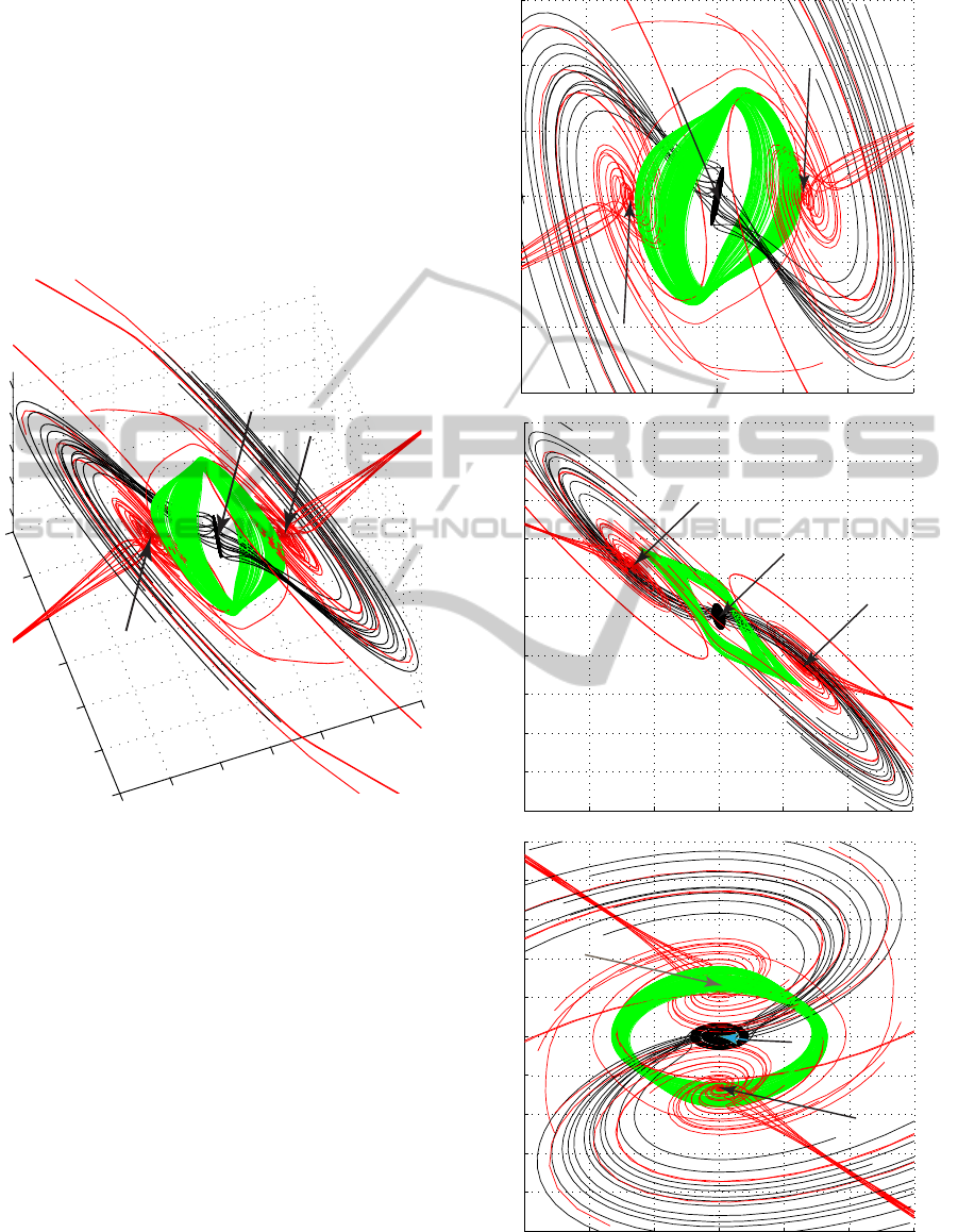
Figure 2: Equilibrium, stable manifolds of saddles, and lo-
calization of hidden attractor.
The considered system has three stationary points:
the stable zero point F
0
and the symmetric saddles S
1
and S
2
. To zero equilibrium F
0
correspond the eigen-
values λ
F
0
1
= −7.9591 and λ
F
0
2,3
= −0.0038± 3.2495i
and to the saddles S
1
and S
2
correspond the eigen-
values λ
S
1,2
1
= 2.2189 and λ
S
1,2
2,3
= −0.9915± 2.4066i.
The behavior of trajectories of system in a neighbor-
hood of equilibria is shown in Fig. 3.
We remark that here positive Lyapunov exponent
(Leonov & Kuznetsov, 2007) corresponds to the com-
puted trajectories.
By the above and with provision for the remark on
the existence, in system, of locally stable zero equi-
librium and two saddle equilibria, we arrive at the
conclusion that in A
hidden
a hidden strange attractor
is computed.
−15 −10 −5 0 5 10 15
−3
−2
−1
0
1
2
3
x
y
S
2
S
1
F
0
−15 −10 −5 0 5 10 15
−25
−20
−15
−10
−5
0
5
10
15
20
25
x
z
S
2
F
0
S
1
−3 −2 −1 0 1 2 3
−25
−20
−15
−10
−5
0
5
10
15
20
25
y
E
z
S
1
F
0
S
2
Figure 3: Hidden attractor projections on (x,y), (x,z), and
(y,z).
ICINCO 2011 - 8th International Conference on Informatics in Control, Automation and Robotics
282

4 CONCLUSIONS
In the present work the application of special
analytical-numerical algorithm for hidden attractor
localization is discussed. The existence of such hid-
den attractor in classical Chua’s circuits is demon-
strated.
It is also can be noted that to obtain existence of
hidden attractor in Chua’s circuit one can artificially
stabilized (Suykens et al., 1997; Savaci & Gunel,
2006; Leonov et. al., 2010a) zero stationary point
by inserting small stable zone around zero stationary
point into nonlinearity (Chua diode characteristics).
ACKNOWLEDGEMENTS
This work was supported by the Academy of Finland,
the Ministry of Education and Science (Russia), and
Saint-Petersburg State University.
REFERENCES
Lorenz E. N. (1963). Deterministic nonperiodic flow. J.
Atmos. Sci. V.20. pp. 130–141.
Rossler O. E. (1976). An Equation for Continuous Chaos.
Physics Letters. V.57A. N5. pp. 397–398.
Chua L. O., Lin G. N. (1990). Canonical Realization of
Chua’s Circuit Family. IEEE Transactions on Circuits
and Systems. V.37. N4. pp. 885–902.
Chen G. & Ueta T. (1999). Yet another chaotic attractor.
Int. J. Bifurcation and Chaos. N9, pp. 1465–1466.
Leonov G. A., Kuznetsov N. V., Vagaytsev V. I.
(2011). Localization of hidden Chua’s attrac-
tors. Physics Letters A. 375 (35), pp. 2230-2233
(doi:10.1016/j.physleta.2011.04.037)
Leonov G. A. (2009). On the method of harmonic lineariza-
tion. Automation and remote controle. 70(5), pp. 800–
810.
Leonov G. A. (2009). On the Aizerman problem. Automa-
tion and remote control. 70(7), pp. 1120–1131.
Leonov G. A. (2010). Effective methods for periodic os-
cillations search in dynamical systems. App. math. &
mech. 74(1), pp. 24–50.
Leonov G. A., Vagaitsev V. I., Kuznetsov N. V. (2010a).
Algorithm for localizing Chua attractors based on the
harmonic linearization method. Doklady Mathemat-
ics. 82(1), pp. 663–666.
Leonov G. A., Bragin V. O., Kuznetsov N. V. (2010b).
Algorithm for Constructing Counterexamples to the
Kalman Problem. Doklady Mathematics. 82(1),
pp. 540–542.
Kuznetsov N. V., Leonov G. A. (2008). Lyapunov quanti-
ties, limit cycles and strange behavior of trajectories
in two-dimensional quadratic systems. Journal of Vi-
broengineering. Vol. 10, Iss. 4, pp. 460–467.
Leonov G. A., Kuznetsov, N. V. (2010). Limit cycles of
quadratic systems with a perturbed weak focus of or-
der 3 and a saddle equilibrium at infinity Doklady
Mathematics. 82(2), pp. 693–696.
Leonov G. A., Kuznetsov N. V., and Kudryashova E. V.
(2011). A Direct Method for Calculating Lyapunov
Quantities of Two-Dimensional Dynamical Systems.
Proceedings of the Steklov Institute Of Mathematics.
Vol. 272 (SUPPL. 1), pp. S119–S127.
Chua L. O. (1992). A Zoo of Strange Attractors from the
Canonical Chua’s Circuits. Proceedings of the IEEE
35th Midwest Symposium on Circuits and Systems
(Cat. No.92CH3099-9). V.2. pp. 916–926.
Chua L. O. (1995). A Glimpse of Nonlinear Phenomena
from Chua’s Oscillator. Philosophical Transactions:
Physical Sciences and Engineering. V.353. N1701.
pp. 3–12.
Bilotta E., Pantano P. (2008). A gallery of Chua attractors.
World scientific series on nonlinear science, Series A.
Shi Z., Hong S., and Chen K. (2008). Experimental study on
tracking the state of analog Chua’s circuit with particle
filter for chaos synchronization. Physics Letters A,
Vol. 372, Iss. 34, pp. 5575–5580.
Leonov G. A., Kuznetsov N. V. (2007). Time-Varying Lin-
earization and the Perron effects. International Journal
of Bifurcation and Chaos. Vol. 17, No. 4, pp. 1079–
1107.
Savaci F. A., Gunel S. (2006). Harmonic Balance Analy-
sis of the Generalized Chua’s Circuit. International
Journal of Bifurcation and Chaos. Vol. 16, No. 8,
pp. 2325–2332.
Suykens J. A. K., Huang A., Chua L. O. (1997). AFamily of
n-scroll Attractors from a Generalized Chuas Circuit.
AEU-International Journal of Electronics & Commu-
nications. Vol. 51, No. 3, pp. 131–138.
HIDDEN ATTRACTOR IN CHUA'S CIRCUITS
283