SKELETAL ALGORITHMS
Michal R. Przybylek
Faculty of Mathematics, Informatics and Mechanics, University of Warsaw, Warsaw, Poland
Keywords:
Evolutionary algorithms, Process mining, Language recognition, Minimum description length.
Abstract:
This paper introduces a new kind of evolutionary method, called “skeletal algorithm”, and shows its sam-
ple application to process mining. The basic idea behind the skeletal algorithm is to express a problem in
terms of congruences on a structure, build an initial set of congruences, and improve it by taking limited
unions/intersections, until a suitable condition is reached. Skeletal algorithms naturally arise in the context of
data/process minig, where the skeleton is the “free” structure on initial data and a congruence corresponds to
similarities in data. In such a context, skeletal algorithms come equipped with fitness functions measuring the
complexity of a model. We examine two fitness functions for our sample problem — one based on Minimum
Description Length Principle, and the other based on Bayesian Interpretation.
1 INTRODUCTION
The idea of evolutionary computing dates back to the
late 1950, when it was first introduced by Bremer-
mann in (Bremermann, 1962), Friedberg, Dunham
and North (Friedberg, 1956; Friedberg et al., 1959),
and then developed by Rechenberg in (Rechenberg,
1971), and Holland in (Holland, 1975). Skeletal algo-
rithm derives its foundations from these methods and
creates a new branch of evolutionary metaheuristics
concerned on data and process mining. The crucial
observation that leads to skeletal algorithms bases on
Minimum Description Length Principle (Grunwald
and Rissanen, 2007), which among other things, says
that the task of finding “the best model” describing
given data is all about discovering similarities in the
data. Thus, when we start from a model that fully de-
scribes the data (i.e. the skeletal model of the data),
but does not see any similarities, we may obtain a
“better model” by unifying some parts of that model.
Unifying parts of a model means just taking a quotient
of that model, or equally — finding a congruence re-
lation.
1.1 Process Mining
Process mining (van der Aalst, 2011; Weijters and
van der Aalst, 2001; de Medeiros et al., 2004; van der
Aalst et al., 2000; van der Aalst and ter Hofstede,
2002; van der Aalst et al., 2006b; Wynn et al.,
2004; van der Aalst et al., 2006a; van der Aalst and
M. Pesic, 2009) is a new and prosperous technique
that allows for extracting a model of a business pro-
cess based on information gathered during real execu-
tions of the process. The methods of process mining
are used when there is no enough information about
processes (i.e. there is no a priori model), or there is a
need to check whether the current model reflects the
real situation (i.e. there is a priori model, but of a du-
bious quality). One of the crucial advantages of pro-
cess mining over other methods is its objectiveness —
models discovered from real executions of a process
are all about the real situation as it takes place, and
not about how people think of the process, and how
they wish the process would be like. In this case, the
extracted knowledge about a business process may be
used to reorganize the process to reduce its time and
cost for the enterprise.
Table 1 shows a typical event-log gathered during
executions of the process to determine and identify a
possible disease or disorder of a patient. In this paper,
we assume that with every such an event-log there are
associated:
• an identifier referring to the execution (the case)
of the process that generated the event
• a unique timestamp indicating the particular mo-
ment when the event occurred
• an observable action of the event; we shall as-
sume, that we are given only some rough infor-
mation about the real actions.
and we shall forget about any additional information
80
R. Przybylek M..
SKELETAL ALGORITHMS.
DOI: 10.5220/0003674700800089
In Proceedings of the International Conference on Evolutionary Computation Theory and Applications (ECTA-2011), pages 80-89
ISBN: 978-989-8425-83-6
Copyright
c
 2011 SCITEPRESS (Science and Technology Publications, Lda.)

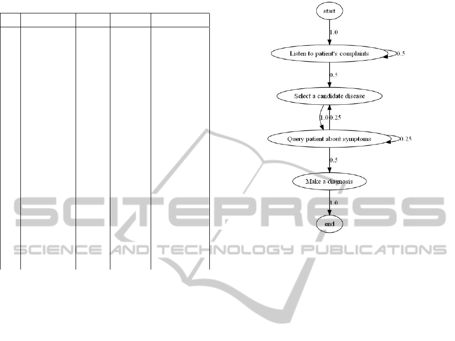
Table 1: An event log.
Case Observable
Action
Actor Timestamp Data
127 START Dr. Moor 11:30:52
07.02.2011
127 Listen to patient’s
complaints
Dr. Moor 11:34:27
07.02.2011
headache
127 Listen to patient’s
complaints
Dr. Moor 11:35:59
07.02.2011
fever
107 START Dr. No 11:36:50
07.02.2011
127 Listen to patient’s
complaints
Dr. Moor 11:39:33
07.02.2011
catarrh
107 Listen to patient’s
complaints
Dr. No 11:39:37
07.02.2011
pain in the left foot
127 Select a candidate
disease
Dr. Moor 11:58:30
07.02.2011
angina
127 Query patient
about symptoms
Dr. Moor 12:01:11
07.02.2011
sore throat? — yes
127 Query patient
about symptoms
Dr. Moor 12:08:21
07.02.2011
white patches on
the tonsils? — yes
107 Select a candidate
disease
Dr. No 12:10:31
07.02.2011
broken leg
107 Query patient
about symptoms
Dr. No 12:11:01
07.02.2011
swollen leg? — No
107 Select a candidate
disease
Dr. No 12:11:33
07.02.2011
joint dislocation
107 Query patient
about symptoms
Dr. No 12:14:00
07.02.2011
blood inflamma-
tion? — Yes
107 Make a diagnosis Dr. No 12:16:02
07.02.2011
joint dislocation
107 END Dr. No 12:16:50
07.02.2011
127 Make a diagnosis Dr. Moor 12:34:01
07.02.2011
angina
127 END Dr. Moor 12:34:55
07.02.2011
... ... ... ... ...
and attributes associated with an execution of a pro-
cess. The first property says that we may divide a
list of events on collections of events corresponding
to executions of the process, and the second property
let us linearly order each of the collections. If we
use only information about the relative occurrences
of two events (that is: which of the events was first,
and which was second), then the log may be equally
described as a finite list of finite sequences over the
set ObservableAction of all possible observable ac-
tions. Therefore we may think of the log as a fi-
nite sample of a probabilistic language over alpha-
bet ObservableAction — or more accurately — as
the image of a finite sample of a probabilistic lan-
guage over Action under a morphism h : Action →
ObservableAction. The morphism h describes our im-
perfect information about the real actions. In the ex-
ample from table 1 (here we use the first letter of the
name of an action as abbreviate for the action)
ObservableAction = {l, s,q,m}
and the sample contains sequences
S = {hl,l,l,s,q,q,mi,hl,s,q,s,q,mi} (1)
Figure 1 shows a model recognized from this sample.
Here Action = ObservableAction and h is the identity
morphism (there are no duplicated events).
Figure 1: Model mined from Table 1.
1.2 A Survey of Most Successful Process
Mining Methods
1. Algorithms α, α
++
,β (van der Aalst and van Don-
gen, 2002)(Wen et al., 2006)(Ren et al., 2007).
They are able to mine models having single tasks
only. These algorithms base on finding causalities
of tasks.
2. Genetic algorithms (van der Aalst et al.,
2006a)(Medeiros et al., 2007). Models are tran-
sition matrices of Petri nets. A crossing operation
exchanges fragments of the involved matrices.
3. Algorithms based on prefix trees (Cook and
Woolf, 1998). The prefix tree is built for a given
set of executions of a process. Learning corre-
sponds to finding a congruence on the tree.
4. Algorithms based on regular expressions
(Brazma, 1994). Models are regular expressions.
Learning corresponds to a compression of the
regular expression.
5. Statistical methods based on recursive neural net-
works (Cook and Woolf, 1998). The model is rep-
resented by a three-layer neural network. The hid-
den layer corresponds to the states of discovered
automaton.
6. Statistical methods based on Markov chains
(Cook and Woolf, 1998), or Stochastic Activation
Graphs (Herbst, 2000). The set of executions of a
process is assumed to be a trajectory of a Markov
SKELETAL ALGORITHMS
81

chain; such a Markov chain is then constructed
and turned into finite state machine by pruning
transitions that have small probabilities or insuf-
ficient support.
Skeletal algorithms reassembles and generalizes the
idea from algorithms based on prefix trees and regu-
lar expressions, and makes the task of finding a con-
gruence structured and less ad hoc. We will elaborate
more on skeletal algorithms in the next section.
1.3 Organization of the Paper
We assume that the reader is familiar with basic math-
ematical concepts. The paper is structured as fol-
lows. In section 2 we shall briefly recall some crucial
for this paper mathematical concepts, and introduce
skeletal algorithms. Section 3 describes our approach
to process mining via skeletal algorithms. In section 4
we show some examples of process mining. We con-
clude the paper in section 5.
2 SKELETAL ALGORITHMS
Skeletal algorithms are a new branch of evolution-
ary metaheuristics focused on data and process min-
ing. The basic idea behind the skeletal algorithm is
to express a problem in terms of congruences on a
structure, build an initial set of congruences, and im-
prove it by taking limited unions/intersections, until
a suitable condition is reached. Skeletal algorithms
naturally arise in the context of data/process mining,
where the skeleton is the “free” structure on initial
data and a congruence corresponds to similarities in
the data. In such a context, skeletal algorithms come
equipped with fitness functions measuring the com-
plexity of a model.
Skeletal algorithms, search for a solution of a
problem in the set of quotients of a given structure
called the skeleton of the problem. More formally, let
S be a set, and denote by Eq(S) the set of equivalence
relations on S. If i ∈ S is any element, and A ∈ Eq(S)
then by [i]
A
we shall denote the abstraction class of i
in A — i.e. the set {j ∈ S : jAi}. We shall consider
the following skeletal operations on Eq(S):
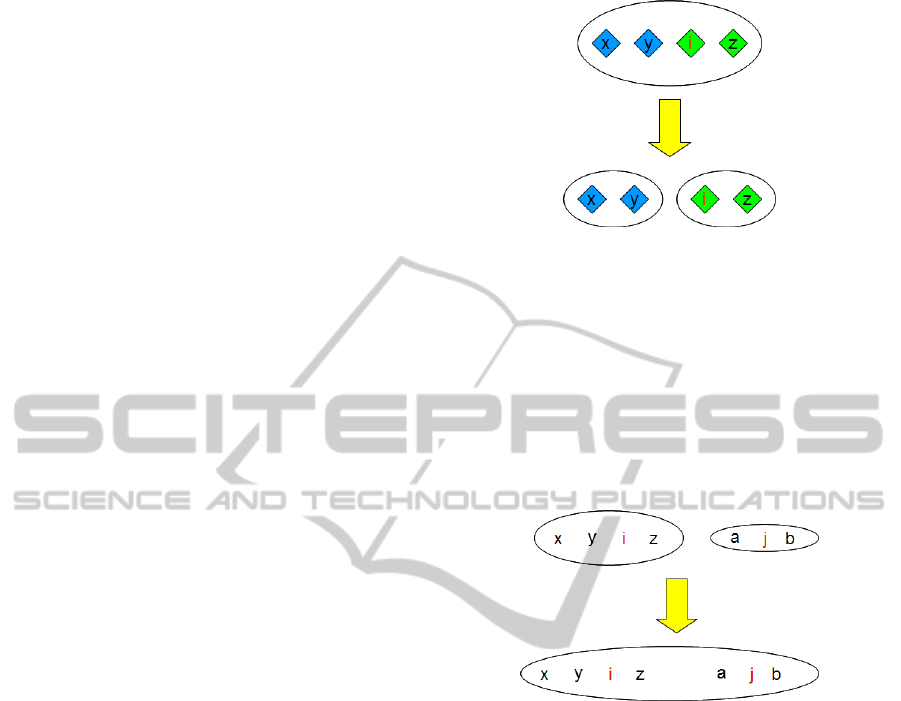
1. Splitting
The operation split : {0,1}
S
×S ×Eq(S) →Eq(S)
takes a predicate P: S →{0,1}, an element i ∈ S,
an equivalence relation A ∈ Eq(S) and gives the
largest equivalence relation R contained in A and
satisfying: ∀
j∈[i]
A
iR j ⇒ P(i) = P( j). That is —
it splits the equivalence class [i]
A
on two classes:
one for the elements that satisfy P and the other of
the elements that do not (Figure 2).
Figure 2: Equivalence class [i] is split according to the pred-
icate: blue elements satisfies the predicate, whereas green
— not.
2. Summing
The operation sum : S ×S ×Eq(S) → Eq(S) takes
two elements i, j ∈ S, an equivalence relation A ∈
Eq(S) and gives the smallest equivalence relation
R satisfying iR j and containing A. That is — it
merges the equivalence class [i]
A
with [ j]
A
(see
Figure 3).
Figure 3: Equivalence classes [i] and [ j] are merged.
3. Union
The operation union: S × Eq(S) × Eq(S) →
Eq(S)×Eq(S) takes one element i ∈S, two equiv-
alence relations A,B ∈ Eq(S) and gives a pair
hR,Qi, where R is the smallest equivalence re-
lation satisfying ∀
j∈[i]
B
iR j and containing A, and
dually Q is the smallest equivalence relation sat-
isfying ∀
j∈[i]
A
iQ j and containing B. That is — it
merges the equivalence class corresponding to an
element in one relation, with all elements taken
from the equivalence class corresponding to the
same element in the other relation (see Figure 4).
4. Intersection
The operation intersection : S ×Eq(S) ×Eq(S) →
Eq(S)×Eq(S) takes one element i ∈S, two equiv-
alence relations A,B ∈ Eq(S) and gives a pair
hR,Qi, where R is the largest equivalence relation
satisfying ∀
x,y∈[i]
A
xRy ⇒x, y ∈[i]
B
∨x, y /∈[i]
B
and
contained in A, and dually Q is the largest equiv-
alence relation satisfying ∀
x,y∈[i]
B
xQy ⇒ x,y ∈
[i]
A
∨x,y /∈[i]
A
and contained in B. That is — it in-
ECTA 2011 - International Conference on Evolutionary Computation Theory and Applications
82

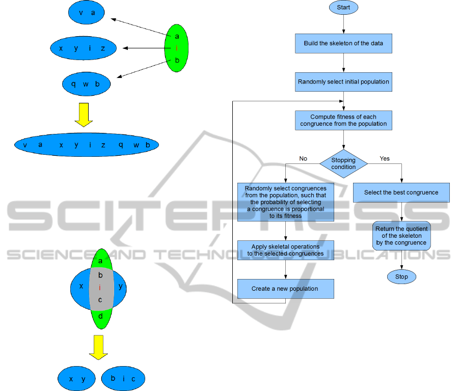
Figure 4: Merging equivalence classes in one relation along
elements from the equivalence class [i] in another relation.
tersects the equivalence class corresponding to an
element in one relation, with the equivalence class
corresponding to the same element in the other re-
lation (see Figure 5).
Figure 5: Spliting the equivalence class of i in one relation
along equivalence class of i in another relation.
Furthermore, we shall assume that there is also a
fitness function ∆: H(S) → R. The general template
of skeletal algorithm is shown on figure 6.
There are many things that can be implemented
differently in various problems.
2.1 Construction of the Skeleton
As pointed out earlier, the skeleton of a problem
should correspond to the “free model” build upon
sample data. Observe, that it is really easy to plug
in the skeleton some priori knowledge about the so-
lution — we have to construct a congruence relation
induced by the priori knowledge and divide by it the
“free unrestricted model”. Also, this suggests the fol-
lowing optimization strategy — if the skeleton of a
problem is too big to efficiently apply the skeletal al-
gorithm, we may divide the skeleton on a family of
Figure 6: Skeletal Algorithm.
smaller skeletons, apply to each of them the skeletal
algorithm to find quotients of the model, glue back the
quotients and apply again the skeletal algorithm to the
glued skeleton.
2.2 Construction of the Initial
Population
Observe that any equivalence relation on a finite set S
may be constructed by successively applying sum op-
erations to the identity relation, and given any equiva-
lence relation on S, we may reach the identity relation
by successively applying split operations. Therefore,
every equivalence relation is constructible from any
equivalence relation with sum and split operations. If
no priori knowledge is available, we may build the ini-
tial population by successively applying to the iden-
tity relation both sum and split operations.
2.3 Selection of Operations
For all operations we have to choose one or more ele-
ments from the skeleton S, and additionally for a split
operation — a splitting predicate P : S → {0,1}. In
most cases these choices have to reflect the structure
SKELETAL ALGORITHMS
83

of the skeleton — i.e. if our models have an alge-
braic or coalgebraic structure, then to obtain a quo-
tient model, we have to divide the skeleton by an
equivalence relation preserving this structure, that is,
by a congruence. The easiest way to obtain a congru-
ence is to choose operations that map congruences to
congruences. Another approach is to allow operations
that move out congruences from they class, but then
“improve them” to congruences, or just punish them
in the intermediate step by the fitness function.
2.4 Choosing Appropriate Fitness
Function
Data nad process mining problems frequently come
equipped with a natural fitness function measuring
the total complexity of data given a particular model.
One of the crucial conditions that such a function has
to satisfy is the ability to easily adjust its value on a
model obtained by applying skeletal operations.
2.5 Creation of Next Population
There is a room for various approaches. We have ex-
perimented most successful with the following strat-
egy — append k-best congruences from the previous
population to the result of operations applied in the
former step of the algorithm.
3 SKELETAL ALGORITHMS IN
PROCESS MINING
If we forget about additional information and at-
tributes associated with an execution of a process,
then the task of identifying a process reduces to the
task of language recognition. The theory of language
recognition that gives most negative results is “identi-
fication of a language in the limit” developed by Mark
Gold (Gold, 1967). The fundamental theorem pub-
lished by Dan Angluin (Angluin, 1980) says that a
class of recursively indexed languages is (recursively)
identifiable in the limit iff for every language L from
the class there exists an effectively computable finite
“tell-tale” — that is: a subset T of L such that: if T is
a subset of any other language K from the class, then
K * L. An easy consequence of this theorem is that
the set of regular languages is not identifiable in the
limit. Another source of results in this context is the
theory of PAC-learning developed by Leslie Valiant
(Valiant, 1984).
Although these results are fairly interesting, in the
context of process mining, we are mostly given a very
small set of sample data, and our task is to find the
most likely hypothesis — the question: “if we were
given sufficiently many data, would it have been pos-
sible to find the best hypothesis?” is not really practi-
cal.
3.1 Probabilistic Languages
A probabilistic language L over an alphabet Σ is any
subset of Σ
∗
×[0,1] that satisfies the following condi-
tion:
∑
hw,pi∈L
p = 1. Note that probabilistic languages
over Σ are the same as probability distributions over
Σ
∗
.
A probabilistic finite state automaton is a quadru-
ple A = hΣ, S,l,δi, where:
• Σ is a finite set called the “alphabet of the automa-
ton”
• S is a finite set of states
• l is a labeling function S → Σ ∪{start, end} such
that l
−1
[start] = {s
start
}6= {s
end
}= l
−1
[end]; state
s
start
is called “the initial state of the automaton”,
and s
end
“the final state of the automaton”
• δ is a transition function S ×S → [0, 1] such that:
– ∀
s∈S
∑
q∈S
δ(s,q) = 1
– ∀
s∈S
δ(s,s
start
) = 0
– δ(s
end
,s
end
) = 1
A trace of an automaton A starting in a state s
0
and
ending in a state s
k
is a sequence hs
1
,. .. ,s
k
i ∈ S
∗
. A
full trace of an automaton is a trace starting in s
start
and ending in s
end
.
In our setting models correspond to probabilistic
finite automata, the distributions are induced by the
probabilities of full traces of the automata, and mor-
phisms map states to they actions (i.e. labels).
3.2 Skeleton
Given a list of sample data K : n = {0,···,n −1} →
Σ
∗
, by a skeleton of K we shall understand the au-
tomaton: skeleton(K) = hΣ,S,l,δi, where:
• S = {hi,ki: i ∈ n, k ∈{1,...,|K(i)|}}∪{−∞,∞}
• l(−∞) = start, l(∞) = end, l(hi,ki) = K(i)
k
,
where the subscript k indicates the k-th element
of the sequence
• δ(−∞,hi,1i) = 1, δ(∞,∞) = 1, δ(hi, |K(i)|i,∞) =
1, δ(hi,ki,hi,k + 1i) = 1
So the skeleton of a list of data is just an automaton
corresponding to this list enriched with two states —
initial and final. This automaton describes the situ-
ation, where all actions are different. Our algorithm
will try to glue some actions that give the same output
ECTA 2011 - International Conference on Evolutionary Computation Theory and Applications
84

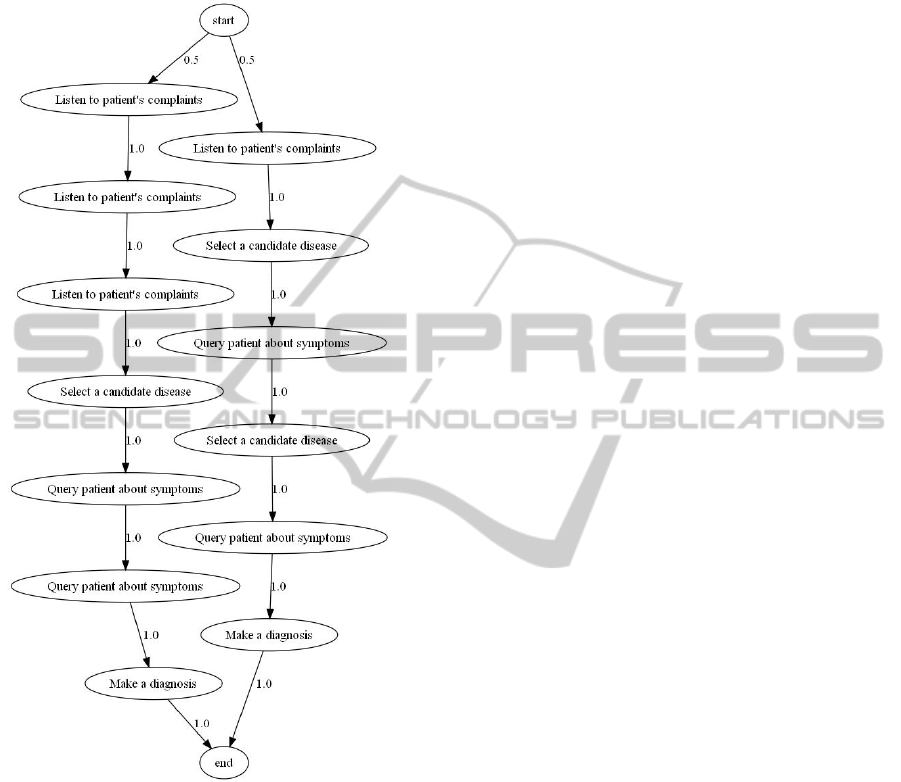
(shall search for the best fitting automaton in the set of
quotients of the skeletal automaton). Figure 7 shows
the skeletal automaton of the sample 1 from section 1.
Figure 7: Skeletal model of the sample 1.
Given a list of sample data K : n → Σ
∗
, our search
space Eq(S) consists of all equivalence relations on S.
3.3 Skeletal Operations
1. Splitting
For a given congruence A, choose randomly a
state hi,ki ∈ skeleton(K) and make use of two
types of predicates
• split by output — P(hj,li) = 1 ⇔
∃
hi
0
,k
0
i∈[hi,ki]
A
δ(hj,li,hi
0
,k
0
i)
• split by input — P(hj,li) = 1 ⇔
∃
hi
0
,k
0
i∈[hi,ki]
A
δ(hi
0
,k
0
i,hj,li)
2. Summing
For a given congruence A, choose randomly two
states hi,ki,hj, li such that l(hi,ki) = l(hj,li).
3. Union/Intersection
Given two skeletons A,B choose randomly a state
hi,ki ∈ skeleton(K).
Let us note that by choosing states and predicates
according to the above description, all skeletal opera-
tions preserve congruences on skeleton(K).
3.4 Fitness
Let v
0
: v = hv
0
,v
1
,··· , v
k
i be a trace of a probabilis-
tic automaton. Assuming that we start in node v
0
,
the probability of moving successively through nodes
v
1
,··· , v
k
is
P(v|v
0
) =
k
∏
i=1
δ(v
i−1
,v
i
)
and it give us a probability distribution on S
k
:
P(v) =
∑
v
0
∈S
µ(v
0
)P(v|v
0
)
where µ is any probability distribution on the states
S of the automaton. If we choose for µ a probabil-
ity mass distribution concentrated in a single node v
0
,
then P(v) would depend multiplicatively on proba-
bilistic transitions P(v
i−1
,v
i
). In this case any local
changes in the structure of the automaton (like split-
ting or joining nodes) give multiplicative perturba-
tions on the probability P(v), so it is relatively easy
(proportional to the number of affected nodes) to up-
date the complexity of v.
Consider any full trace v = hv
0
=
start, v
1
,··· , v
k
= endi of an automaton. Ac-
cording to our observation, we may associate with it
the following probability:
P(v) =
k
∏
i=1
δ(v
i−1
,v
i
) =
∏
x∈S
∏
a∈S
δ(x,a)
|{i: x=v
i
∧a=v
i
+1}|
where for every x the term
∏
a∈S
δ(x,a)
|{i: x=v
i
∧a=v
i
+1}|
depends only on the
number of pass to the state a. Hence, we may restrict
our analysis to single states.
Let s be such a state with l output probabilis-
tic transitions a
1
,··· , a
l
, and let us assume that the
probability of passing the j-th arrow is p
j
. Then the
probability of consecutively moving through arrows
x = ha
i
1
,··· , a
i
k
i when visiting node s is:
p
s
(x) =
k
∏
j=1
p
i
j
=
l
∏
j=1
p
c
j
j
SKELETAL ALGORITHMS
85

where c
j
is the number of occurences of a
j
in x. Thus,
given a sample x and a probabilistic node s the optimal
length of a code describing x is about
log(
1
p
s
(x)
)
and the shortest code is achieved for s having proba-
bilities
p
1
=
c
1
k
,··· , p
k
=
c
l
k
Now, let us assume that we do not know probabil-
ities at s. Then any code describing x via s has to
contain some information about these probabilities.
A “uniform approach” would look like follows: for
a given sample x chose the optimal probability node
s
x
, then opt(x) = p
s
x
(x) is not a probability on l
k
as
it does not sum up to 1 (i.e. it does not contain in-
formation about choosing appropriate hypothesis s
x
);
however
mdl(x) =
opt(x)
∑
x∈l
k
opt(x)
= (
∑
r
1
+···+r
l
=k

k
r
1
,··· , r
l

l
∏
i=1
r
r
i
i
)
−1
l
∏
i=1
c
c
i
i
= m
l
∏
i=1
c
c
i
i
(2)
is, where

k
r
1
,···,r
l

is the multionomial k over
r
1
,··· , r
l
. One may take another approach based on
Bayesian interpretation. Let us fix a meta-distribution
q on all probabilistic nodes s having the same out-
put arrows. This distribution chooses probabilities
p
1
,··· , p
l
, that is — non-negative real numbers such
that p
1
+ ···+ p
l
= 1 — then for a given sample x
chose a node s
p
1
,···,p
l
with probability q(s
p
1
,···,p
l
) and
describe x according to that node:
bayes(x) =
Z
p
1
+···+p
l
=1,p
i
≥0
p
s
p
1
,···,p
l
(x)q(s
p
1
,···,p
l
)
If q is a uniform distribution, then
bayes(x) =
R
p
1
+···+p
l
=1,p
i
≥0
∏
l
i=1
p
c
i
i
Vol(∆
l
)
=
Γ(l)
∏
l
i=1
Γ(c
i
+ 1)
Γ(
∑
l
i=1
(c
i
+ 1))
=
Γ(l)
Γ(k + l)
l
∏
i=1
c
c
i
i
= b
l
∏
i=1
c
c
i
i
(3)
So, mdl(x) = m
∏
l
i=1
c
c
i
i
and bayes(x) = b
∏
l
i=1
c
c
i
i
,
where m,b are constants making mdl and bayes prob-
ability distributions. In fact, these distributions are
really close — by using Striling’s formula
n
n
≈
√
2πn(
n
e
)
n
we have
bayes(x) ≈ b
0
l
∏
i=1
c
c
i
+
1
2
i
where b
0
= be
−n
(2π)
l/2
is just another constant. We
shall prefer the Bayesian distribution as it is much
easier to compute and update after local changes, but
we should be aware that it slightly more favors ran-
dom sequences than the optimal (in the sense of min-
imum regret) distribution.
The total distribution on traces is then given by:
bayes
trace
(v) =
∏
s∈S
bayes
s
(v ↓ s)
where bayes
s
is the Bayesian distribution correspond-
ing to the node s and v ↓s is the maximal subsequence
of v consisting of elements directly following s. And
the corresponding complexity of v is:
comp(v) = −
∑
s∈S
log(bayes
s
(v ↓ s))
Although this complexity assumes that we do not
know the exact probabilities of the automaton, it also
assumes that we know all its other properities. Our
research showed that the other aspects of the automa-
ton are best described with two-parts codes. Thus, the
fitness function for a congruence A on the skeleton
of sample data K : n → Σ
∗
would be proportional to
the sum of the description (neglecting probabilities)
of the quotient model skeleton(K)/A and complexi-
ties of each K(i) according to that model:
∆(A) = −|skeleton(K)/A|−
n−1
∑
i=0
comp
skeleton(K)/A
(K(i))
where |skeleton(K)/A| may be tuned for particular
samples. Our experience showed that choosing
clog(|S|)|{hx,yi ∈ S ×S : δ(x,y) > 0}|
for a small constant c > 1 behaves best.
4 EXAMPLES
4.1 Non-deterministic Automata
Given a non-deterministic automata like on figure 8
we generate sample of n words by moving through
each arrow outgoing from a state with equal probabil-
ities. Figure 9 shows discovered model after seeing 4
samples, Figure 10 after seeing 16, and figure 11 after
seeing 160 samples. Note, that the automaton is redis-
covered with a great precision after seeing a relatively
small sample data.
ECTA 2011 - International Conference on Evolutionary Computation Theory and Applications
86

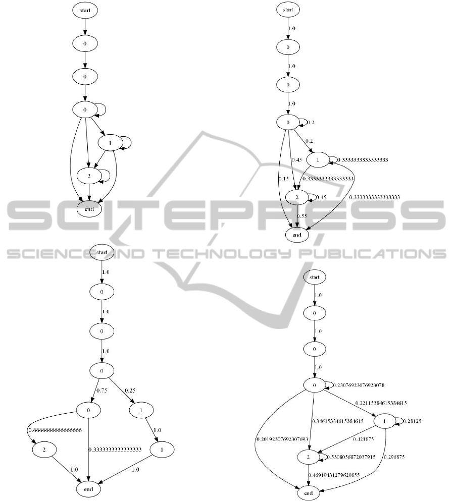
Figure 8: Non-deterministic automaton.
Figure 9: Model discovered after seeing 4 samples.
4.2 Testing Sample
In this example we use samples from (Cook and
Woolf, 1998):
L1 = A,B,C, A,B,C,B,A,C,B,A,C,A,
B,C,B, A,C,B,A,C, A,B,C, B,A,
C, A,B,C, A,B,C,B,A,C,B,A (4)
Figure 10: Model discovered after seeing 16 samples.
Figure 11: Model discovered after seeing 160 samples.
L2 = A,B,C, D,C,E,F,G,H,G,I,J,
G,I,K, L,M, N,O,P,R,F, G,I,
K,L,M,N,O,P,Q, S (5)
Figures 12 and 13 show models discovered from sam-
ple L1 and L2 respectively. Model 12 corresponds
to the model mined by KTAIL method, whereas
model 13 outperforms overfitted RNET, MARKOV
and KTAIL.
SKELETAL ALGORITHMS
87

Figure 12: Model discovered from sample L1.
4.3 Prime Numbers
In this example we show how skeletal algorithms can
learn from a probabilistic source p that does not corre-
spond to any model. We define p to be non-zero only
on prime numbers, and such that the probability for
a given prime number is proportional to its numbers
of bits in binary representation. Figure 14 shows dis-
covered automaton from 500 samples. Observe that it
quite accuratly predicts all 5-bits prime numbers.
5 CONCLUSIONS
In this paper we introduced a new kind of evolution-
ary method — “skeletal algorithm”, especially suit-
able in the context of data and process mining. In such
a context “skeletal algorithms” come often equipped
with a natural fitness function measuring the com-
plexity of a model. We showed a sample application
of “skeletal algorithms” to process mining and ex-
amined two naturally fitness functions — one based
on Minimum Description Length Principle, and an-
other based on Bayesian Interpretation. Although,
obtained results are really promising, there are issues
that should be addressed in future works. The main
concern is to extend the concept of models — our
models base on probabilistic automata, and so the al-
gorithm is not able to mine nodes corresponding to
parallel executions of a process (i.e. AND-nodes).
Also, we are interested in applying various optimiza-
tion techniques and investigate more industrial data.
Figure 13: Model discovered from sample L2.
ECTA 2011 - International Conference on Evolutionary Computation Theory and Applications
88

Figure 14: Prime numbers.
REFERENCES
Angluin, D. (1980). Inductive inference of formal lan-
guages from positive data. In Information and Con-
trol, volume 42.
Brazma, A. (1994). Efficient algorithm for learning simple
regular expressions from noisy examples. In Work-
shop on Algorithmic Learning Theory ALT’94, Lec-
ture Notes in Computer Science, volume 872.
Bremermann, H. J. (1962). Optimization through evolution
and recombination. In Self-Organizing systems 1962,
edited M.C. Yovitts et al., page 93106, Washington.
Spartan Books.
Cook, J. and Woolf, A. (1998). Discovering models of
software processes from event-based data. In ACM
Transactions on Software Engineering and Methodol-
ogy, volume 7/3.
de Medeiros, A., van Dongen, B., van der Aalst, W., and
Weijters, A. (2004). Process mining: Extending the
alpha-algorithm to mine short loops. In BETA Work-
ing Paper Series, Eindhoven. Eindhoven University of
Technology.
Friedberg, R. M. (1956). A learning machines part i. In IBM
Journal of Research and Development, volume 2.
Friedberg, R. M., Dunham, B., and North, J. H. (1959). A
learning machines part ii. In IBM Journal of Research
and Development, volume 3.
Gold, E. (1967). Language identification in the limit. In
Information and Control, volume 10.
Grunwald, P. D. and Rissanen, J. (2007). The minimum
description length principle. In Adaptive Computation
and Machine Learning series. The MIT Press.
Herbst, J. (2000). A machine learning approach to workflow
management. In 11th European Conference on Ma-
chine Learning, Lecture Notes in Computer Science,
volume 1810.
Holland, J. H. (1975). Adaption in natural and artificial sys-
tems. Ann Arbor. The University of Michigan Press.
Medeiros, A., Weijters, A., and van der Aalst, W. (2007).
Genetic process mining: an experimental evaluation.
In Data Mining and Knowledge Discovery, volume
14/2.
Rechenberg, I. (1971). Evolutions strategie – optimierung
technischer systeme nach prinzipien der biologischen
evolution. In PhD thesis. Reprinted by Fromman-
Holzboog (1973).
Ren, C., Wen, L., Dong, J., Ding, H., Wang, W., and Qiu,
M. (2007). A novel approach for process mining based
on event types. In IEEE SCC 2007, pages 721–722.
Valiant, L. (1984). A theory of the learnable. In Communi-
cations of The ACM, volume 27.
van der Aalst, W. (2011). Process mining: Discovery,
conformance and enhancement of business processes.
Springer Verlag.
van der Aalst, W., de Medeiros, A. A., and Weijters, A.
(2006a). Process equivalence in the context of genetic
mining. In BPM Center Report BPM-06-15, BPMcen-
ter.org.
van der Aalst, W. and M. Pesic, M. S. (2009). Beyond pro-
cess mining: From the past to present and future. In
BPM Center Report BPM-09-18, BPMcenter.org.
van der Aalst, W. and ter Hofstede, A. (2002). Workflow
patterns: On the expressive power of (petri-net-based)
workflow languages. In BPM Center Report BPM-02-
02, BPMcenter.org.
van der Aalst, W., ter Hofstede, A., Kiepuszewski, B., and
Barros, A. (2000). Workflow patterns. In BPM Center
Report BPM-00-02, BPMcenter.org.
van der Aalst, W. and van Dongen, B. (2002). Discover-
ing workflow performance models from timed logs.
In Engineering and Deployment of Cooperative Infor-
mation Systems, pages 107–110.
van der Aalst, W., Weijters, A., and Maruster, L. (2006b).
Workflow mining: Discovering process models from
event logs. In BPM Center Report BPM-04-06, BPM-
center.org.
Weijters, A. and van der Aalst, W. (2001). Process min-
ing: Discovering workflow models from event-based
data. In Proceedings of the 13th Belgium-Netherlands
Conference on Artificial Intelligence, pages 283–290,
Maastricht. Springer Verlag.
Wen, L., Wang, J., and Sun, J. (2006). Detecting implicit
dependencies between tasks from event logs. In Lec-
ture Notes in Computer Science, volume 3841, pages
591–603.
Wynn, M., Edmond, D., van der Aalst, W., and ter Hofstede,
A. (2004). Achieving a general, formal and decidable
approach to the or-join in workflow using reset nets.
In BPM Center Report BPM-04-05, BPMcenter.org.
SKELETAL ALGORITHMS
89