A GENERALIZATION OF NEGATIVE NORM MODELS IN THE
DISCRETE SETTING
Application to Stripe Denoising
J´erˆome Fehrenbach
1
, Pierre Weiss
1
and Corinne Lorenzo
2
1
Institut de Math´ematiques de Toulouse, Toulouse University, Toulouse, France
2
ITAV, Toulouse canceropole, Toulouse, France
Keywords:
Denoising, Cartoon+texture decomposition, Primal-dual algorithm, Stationary noise, Fluorescence mi-
croscopy.
Abstract:
Starting with a book of Y.Meyer in 2001, negative norm models attracted the attention of the imaging commu-
nity in the last decade. Despite numerous works, these norms seem to have provided only luckwarm results
in practical applications. In this work, we propose a framework and an algorithm to remove stationary noise
from images. This algorithm has numerous practical applications and we show it on 3D data from a newborn
microscope called SPIM. We also show that this model generalizes Meyer’s model and its successors in the
discrete setting and allows to interpret them in a Bayesian framework. It sheds a new light on these models
and allows to pick them according to some a priori knowledge on the texture statistics. Further results are
available on our webpage at http://www.math.univ-toulouse.fr/∼weiss/PagePublications.html.
1 INTRODUCTION
The purpose of this article is to provide variational
models and algorithms in order to remove stationary
noise from images. The models that are proposed here
turn out to be a generalization of the discretized neg-
ative norm models. This allows to analyse them in a
Bayesian framework. By stationary noise, we mean
that the noise is generated by convolving white noise
with a given kernel. The noise thus appears as ”struc-
tured” in the sense that some pattern might be visible,
see Figure 3(b),(c),(d).
This work was primarily motivated by the recent
development of a microscope called Selective Plane
Illumination Microscope (SPIM). The SPIM is a fluo-
rescence microscope which allows to perform optical
sectioning of a specimen, see (Huisken et al., 2004).
One difference with conventional microscopy is that
the fluorescence light is detected at an angle of 90 de-
grees with the illumination axis. This procedure tends
to degrade the images with stripes aligned with the il-
lumination axis, see Figure 5(a). This kind of noise is
well described by a stationary process. The first con-
tribution of this paper is to provide effective denoising
algorithms dedicated to this imaging modality.
It appears that our models generalize the negative
norms models proposed by Y. Meyer (Meyer, 2001).
This work initiated numerous research in the domain
of texture+cartoon decomposition methods (Vese and
Osher, 2003; Osher et al., 2003; Aujol et al., 2006;
Garnett et al., 2007). Meyer’s idea is to decompose an
image into a piecewise smooth component and an os-
cillatory component. The use of a negativenorm k·k
N
to capture oscillating patterns is motivated by the fact
that if (v
n
) converges weakly to 0 then kv
n
k
N
→ 0.
This interpretation is however not really informative
on what kind of textures are well captured by nega-
tive norms. The second contribution of this paper is to
propose a Bayesian interpretation of these models in
the discrete setting. This allows a better understand-
ing of the decomposition models:
• We can associate a probability density functions
(p.d.f.) to the negative norms. This allows
to choose a model depending on some a priori
knowledge on the texture.
• We can synthetize textures which are adapted to
these negative norms.
• The Bayesian interpretation suggests a new
broader and more versatile class of translation in-
variant models used e.g. for SPIM imaging.
Connection to Previous Works. This work shares
flavors with some previous works. In (Aujol et al.,
337
Fehrenbach J., Weiss P. and Lorenzo C. (2012).
A GENERALIZATION OF NEGATIVE NORM MODELS IN THE DISCRETE SETTING - Application to Stripe Denoising.
In Proceedings of the 1st International Conference on Pattern Recognition Applications and Methods, pages 337-342
DOI: 10.5220/0003742603370342
Copyright
c
 SciTePress

2006) the authors present algorithms and results using
similar approaches. However, they do not propose a
Bayesian interpretation and consider a narrower class
of models. An alternative way of decomposing im-
ages was proposed in (Starck et al., 2005). The idea is
to seek components that are sparse in given dictionar-
ies. Different choices for the elementary atoms com-
posing the dictionary will allow to recover different
kind of textures. See (Fadili et al., 2010) for a review
of these methods and a generalization to the decom-
position into an arbitrary number of components.
The main novelties of the present work are:
1. We do not restrict to sparse components, but allow
for a more general class of random processes.
2. Similarly to (Fadili et al., 2010), the texture is de-
scribed through a dictionary. In the present work
each dictionary is composed of a single pattern
shifted in space, ensuring translation invariance.
3. A Bayesian approach takes into account the sta-
tistical nature of textures more precisely.
4. The decomposition problem is recast into a con-
vex optimization problem that is solved with a
recent algorithm (Chambolle and Pock, 2011) al-
lowing to obtain results in an interactive time.
5. Codes are provided on our
webpage http://www.math.univ-
toulouse.fr/∼weiss/PageCodes.html.
Notation: Let u be a gray-scale image. It is com-
posed of n = n
x
× n
y
pixels, and u(x) denotes the in-
tensity at pixel x. The convolution product between u
and v is u∗v. Thediscrete gradientoperator is denoted
∇. Let ϕ : R
n
→ R be a convex closed function (see
(Rockafellar, 1970)). ∂ϕ denotes its sub-differential.
The Fenchel conjugate of ϕ is denoted ϕ
⋆
, and its re-
solvent is defined by:
(Id + ∂ϕ)
−1
(u) = argmin
v∈R
n
ϕ(v) +
1
2
kv− uk
2
2
,
2 NOISE MODEL
Our objective can be formulated as follows: we want
to recover an original image u, given an observed im-
age u
0
= u + b, where b is a sample of some random
process.
The most standard denoising techniques explicitly
or implicitly assume that the noise is the realization of
a random process that is pixelwise independent and
identically distributed (i.e. a white noise). Under
this assumption, the maximum a posteriori (MAP) ap-
proach leads to optimization problems of kind:
Find u ∈ argmin
u∈R
n
J(u) +
∑
x
φ(u(x) − u
0
(x)),
where
1. exp(−φ) is proportional to the p.d.f. of the noise
at each pixel,
2. J(u) is an image prior.
The assumption that the noise is i.i.d. appears too
restrictive in some situations, and is not adapted to
structured noise (see Figures 2 and 3).
The general model of noise considered in this
work is the following:
b =
m
∑
i=1
λ
i
∗ ψ
i
, (1)
where {ψ
i
}
m
i=1
are filters that describe patterns of
noise, and {λ
i
}
m
i=1
are samples of white noise pro-
cesses {Λ
i
}
m
i=1
. Each process Λ
i
is a set of n i.i.d.
random variables with a p.d.f. exp(−φ
i
).
In short, the convolution that appears in the right-
hand side of (1) states that the noise b is composed of
a certain number of patterns ψ
1
,.. . ,ψ
m
that are repli-
cated in space. The noise b in (1) is a wide sense sta-
tionary noise (Shiryaev, 1996). Examples of noises
that can be generated using this model are shown in
Figure 3.
1. example (b) is a Gaussian white noise. It is
the convolution of a Gaussian white noise with a
Dirac delta function.
2. example (c) is a sine function in the x direction.
It is a sample of a uniform white noise in [−1,1]
convolved with the filter that is constant equal to
1/n
y
in the first column and zero otherwise.
3. example (d) is composed of a single pattern that is
located at random places. It is the convolution of a
sample of a Bernoulli process with the elementary
pattern.
3 RESTORATION ALGORITHM
The Bayesian approach requires a p.d.f. on the space
of images. We assume that the probability of an im-
age u reads p(u) ∝ exp(−J(u)). In this work we will
consider priors of the form:
J(u) = αk∇uk
1,ε
,
where α > 0 is a fixed parameter and if q = (q
1
,q
2
) ∈
R
n×2
, kqk
1,ε
=
∑
x
f
ε

q
q
1
(x)
2
+ q
2
(x)
2

, with
f
ε
(t) =

|t| if |t| ≥ ε
|t|
2
/2ε+ ε/2 otherwise.
ICPRAM 2012 - International Conference on Pattern Recognition Applications and Methods
338

Note that lim
ε→0
k∇uk
1,ε
= TV(u) is the discrete total
variation of u, and that lim
ε→+∞
εk∇uk
1,ε
=
1
2
k∇uk
2
2
up
to an additive constant. This model thus includes TV
and H
1
regularizations as limit cases.
The maximum a posteriori approach in a Bayesian
framework leads to retrieve the image u and the
weights {λ
i
}
m
i=1
that maximize the conditional proba-
bility
p(u,λ
1
,..., λ
m
|u
0
) =
p(u
0
|u,λ
1
,..., λ
m
)p(u,λ
1
,..., λ
m
)
p(u
0
)
.
By assuming that the image u and the noise
components λ
i
are samples of independent pro-
cesses, standard arguments show that maximizing
p(u,λ
1
,...,λ
m
|u
0
) amounts to solving the following
minimization problem:
Find {λ
⋆
i
}
m
i=1
∈ argmin
{λ
i
}
m
i=1
m
∑
i=1
φ
i
(λ
i
) + F(∇(
m
∑
i=1
λ
i
∗ ψ
i
)),
(2)
where
F(q) = αk∇u
0
− qk
1,ε
.
The denoised image u
⋆
is then u
⋆
= u
0
−
∑
m
i=1
λ
⋆
i
∗ ψ
i
.
We propose in this work to solve problem (2) with
a primal-dual algorithm developed in (Chambolle and
Pock, 2011). Let A be the following linear operator:
A : R
m×n
→ R
n×2
λ 7→ ∇(
∑
m
i=1
λ
i
∗ ψ
i
).
By denoting
G(λ) =
m
∑
i=1
φ
i
(λ
i
) (3)
problem (2) can be recast as the following convex-
concave saddle-point problem:
min
λ∈R
n×m
max
kqk
∞
≤1
hAλ,qi − F
∗
(q) + G(λ). (4)
We denote ∆(λ, q) the duality gap of this problem
(Rockafellar, 1970). This problem is solved using the
following algorithm (Chambolle and Pock, 2011): In
practice, for a correct choice of inner products and
parameters σ and τ, this algorithm requires around 50
low-cost iterations for ε = 10
−3
. More details will be
provided in a forthcoming research report.
4 BAYESIAN INTERPRETATION
OF THE DISCRETIZED
NEGATIVE NORM MODELS
In the last decade, the texture+cartoon decomposition
models based on negative norms attracted the atten-
tion of the scientific community. These models often
take the following form:
Algorithm 1: Primal-Dual algorithm.
Input:
ε: the desired precision;
(λ
0
,q
0
): a starting point;
Output:
λ
ε
: an approximate solution to problem (4).
begin
n = 0;
¯
λ
0
= λ
0
;
while ∆(λ
n
,q
n
) > ε∆(λ
0
,q
0
) do
q
n+1
= (Id+ σ∂F
∗
)
−1
(q
n
+ σA
¯
λ
n
);
λ
n+1
= (Id+ τ∂G)
−1
(λ
n
− τA
∗
q
n+1
);
¯
λ
n+1
= λ
n+1
+ θ(λ
n+1
− λ
n
);
n = n+ 1;
end
end
inf
u∈BV(Ω),v∈V,u+v=u
0
TV(u) + kvk
N
(5)
where:
• u
0
is an image to decompose as the sum of a
texture v in V and a structure u in the space of
bounded variation functions BV(Ω),
• V is a Sobolev space of negative index,
• k · k
N
is an associated semi-norm.
Y. Meyer’s seminal model consists in taking V =
W
−1,∞
and the following norm:
kvk
N
= kvk
−1,∞
= inf
g∈L
∞
(Ω)
2
,div(g)=v
kgk
∞
.
In the discrete setting the negative norm models
read:
Find (u,g) ∈ argmin kgk
p
+ αk∇uk
1
subject to u
0
= u+ v
v = ∇
T
g
(6)
where u
0
, u and v are in R
n
, g =

g
1
g
2

∈ R
n×2
and
∇
T
g = ∂
T
1
g
1
+ ∂
T
2
g
2
. The operators ∂
1
and ∂
2
denote
the discrete derivatives with respect to both space di-
rections. If p = ∞, we get the discrete Meyer model.
From an experimental point of view, the choices p = 2
and p = 1 seem to provide better practical results
(Vese and Osher, 2003).
In order to show the equivalence of these models
with the ones proposed in Equation (2), we express
the differential operators as convolution products. As
the discrete derivative operators are usually transla-
tion invariant, this reads:
∇
T
g = h
1
∗ g
1
+ h
2
∗ g
2
.
where ∗ denotes the convolution product and h
1
and
h
2
are derivative filters (typically h
1
= (1,−1) and
h
2
=

1
−1

).
A GENERALIZATION OF NEGATIVE NORM MODELS IN THE DISCRETE SETTING - Application to Stripe
Denoising
339

This simple remark leads to an interesting inter-
pretation of g: it represents the coefficients of an im-
age v in a dictionary composed of the vectors h
1
and
h
2
translated in space.
The negative norms models can thus be inter-
preted as decomposition models in a very simple tex-
ture dictionary. Next, let us show that problem (5) can
be interpreted in a MAP formalism.
Let us define a probability density function:
Definition 1 (Negative Norm p.d.f.). Let Γ be a ran-
dom vector in R
n
and Θ be a random vector in
[0,2π]
n
. Let us assume that p(Γ) ∝ exp(−kΓk
p
) and
that Θ has a uniform distribution. These two random
vectors allow to define a third one:
G =

Γcos(Θ)
Γsin(Θ)

.
Now let us show that problem (6) actually corre-
sponds to a MAP decomposition. Let us assume that:
u
0
= u+ v
with u and v realization of independant random vector
such that p(u) ∝ exp(−αk∇uk
1
) and v = ∇
T
g with g
a realization of G. Then the classical Bayes reasoning
leads to the following equations:
argmax
u∈R
n
,v∈R
n
p(u,v|u
0
)
= argmax
u∈R
n
,v∈R
n
p(u
0
|u,v) · p(u, v)
p(u
0
)
= argmax
u+v=u
0
,u∈R
n
,v∈R
n
p(u,v)
p(u
0
)
= argmin
u+v=u
0
,u∈R
n
,v∈R
n
−log(p(v)) − log(p(u))
= argmin
u+v=u
0
,u∈R
n
,v∈R
n
−log(p(v)) + αk∇uk
1
= argmin
u+v=u
0
,u∈R
n
,v=∇
T
g
kgk
p
+ αk∇uk
1
which is exactly problem (6). Also note that the
model above is equivalent to a slight variant of the
model defined in Equation (2) in the case m = 2:
argmin
u+v=u
0
,u∈R
n
,v=∇
T
g
kgk
p
+ αk∇uk
1
= argmin
g=(g
1
,g
2
)∈R
2n
kgk
p
+ αk∇(u
0
− ∇
T
g)k
1
= argmin
(g
1
,g
2
)∈R
2n
G(g
1
,g
2
) + F(∇(u
0
− h
1
∗ g
1
− h
2
∗ g
2
))
where
• G(g
1
,g
2
) =

∑
x
(g
1
(x)
2
+ g
2
(x)
2
)
p/2

1/p
is a
mixed-norm variant of the function G defined in
Equation (3) (Kowalski, 2009),
• F(q) = αkqk
1
,
• the filters h
1
and h
2
are the discrete derivative fil-
ters defined above.
The same reasoning holds for most negative
norms models proposed lately (Meyer, 2001; Aujol
et al., 2006; Vese and Osher, 2003; Osher et al.,
2003; Garnett et al., 2007), and problem (2) actu-
ally generalizes all these models. To our knowledge,
the Chambolle-Pock implementation (Chambolle and
Pock, 2011) proposed here or the ADMM method (Ng
et al., 2010) (for strongly monotone problems) are the
most efficient numerical approaches.
5 NEGATIVE NORM TEXTURE
SYNTHESIS
The MAP approach to negative norm models de-
scribed above also sheds a new light on the kind of
texture appreciated by the negative norms. In order to
synthetize a texture with p.d.f. (1), it suffices to run
the following algorithm:
1. Generate a sample of a uniform random vector θ ∈
[0,2π]
n
.
2. Generate a sample of a random vector γ with p.d.f.
proportional to exp(−kγk
p
).
3. Generate two vectors g
1
= γcos(θ) and g
2
=
γsin(θ).
4. Generate the texture v = ∇
T

g
1
g
2

.
The results of this simple algorithm are presented
in Figure 1.
6 RESULTS OF THE DENOISING
ALGORITHM
6.1 Synthetic Image
The method was validated on a synthetic example,
where a ground truth is available. A synthetic im-
age was created by adding to a cartoon image (a disk)
the sum of 3 different stationary noises. The result-
ing synthetic image is shown in Figure 2. The cartoon
image and the 3 noise components are presented in
Figure 3(a,b,c,d). The first noise component is a sam-
ple of a Gaussian white noise. The second component
is a sine function in the horizontal direction. The third
component is the sum of elementary patterns, this is
a sample of a Bernoulli law with probability 5.10
−4
convolved with an elementary filter.
ICPRAM 2012 - International Conference on Pattern Recognition Applications and Methods
340

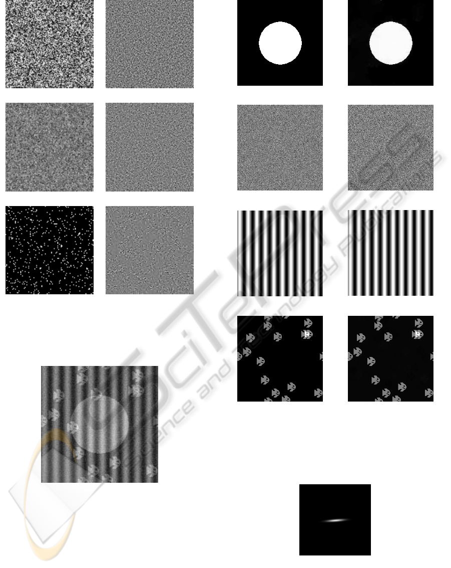
p = 2
p = 1
p = ∞
Figure 1: Left: standard noises. Right: different tex-
tures synthetized with the negative norm p.d.f. Note: we
synthetize the “Laplace” noise by approximating it with a
Bernoulli process.
Figure 2: Synthetic image used for the toy example.
The results of Algorithm 1 are presented in Figure
3(e,f,g,h). The decomposition is almost perfect. This
example is a good proof of concept.
6.2 Real SPIM Image
Algorithm 1 was applied to a zebrafish embryo image
obtained using the SPIM microscope. Two filters ψ
1
and ψ
2
were used to denoise this image. The first filter
ψ
1
is a Dirac (which allows the recovery of Gaussian
(a) (e)
(b) (f)
(c)
(g)
(d) (h)
Figure 3: Toy example. Left column: real components;
right column: estimated components using our algorithm.
(a,e): cartoon component - (b,f): Gaussian noise, std 0.2 -
(c,g): Stripes component (sine)- (d,h): ’Poisson’ noise com-
ponent (poisson means fish in French).
Figure 4: A detailed view of filter ψ
2
.
white noise), and the second filter ψ
2
is an anisotropic
Gabor filter with principal axis directed by the stripes
(this orientation was obtained by user). The filter ψ
2
is shown in Figure 4.
A GENERALIZATION OF NEGATIVE NORM MODELS IN THE DISCRETE SETTING - Application to Stripe
Denoising
341

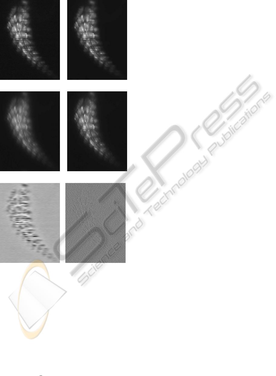
(a) (d)
(b) (e)
(c) (f)
Figure 5: Top-Left: original image zebrafish embryo
Tg.SMYH1:GFP Slow myosin Chain I specific fibers - Top-
Right: TV-L2 denoising - Mid-Left: H
1
-Gabor restoration
- Mid-Right: TV-Gabor restoration - Bottom-Left: stripes
identified by our algorithm - Bottom-Right: white noise.
The original image is presented in Figure 5(a), and
the result of Algorithm 1 is presented in Figure 5(e).
We also present a comparison with two other algo-
rithms in Figures 5(d,b):
• a standard TV-L
2
denoising algorithm. The algo-
rithm is unable to remove the stripes as the prior
is unadapted to the noise.
• an “H
1
-Gabor” algorithm which consists in set-
ting F(·) =
1
2
k · k
2
2
in equation (2). The image
prior thus promotes smooth solutions and pro-
vides blurry results.
ACKNOWLEDGEMENTS
The authors wish to thank Julie Batut for providing
the images of the zebrafish. They also thank Val´erie
Lobjois, Bernard Ducommun, Raphael Jorand and
Franc¸ois De Vieilleville for their support during this
work.
REFERENCES
Aujol, J.-F., Gilboa, G., Chan, T., and Osher, S. (2006).
Structure-texture image decomposition - modeling, al-
gorithms, and parameter selection. Int. J. Comput. Vi-
sion, vol. 67(1), pp. 111-136.
Chambolle, A. and Pock, T. (2011). A first-order primal-
dual algorithm for convex problems with applications
to imaging. J. Math. Imaging Vis. 40(1): 120-145.
Fadili, M., Starck, J.-L., Bobin, J., and Moudden, Y. (2010).
Image decomposition and separation using sparse rep-
resentations: an overview. Proc. of the IEEE, Spe-
cial Issue: Applications of Sparse Representation, vol.
98(6), pp. 983-994,.
Garnett, J., Le, T., Meyer, Y., and Vese, L. (2007). Image
decompositions using bounded variation and general-
ized homogeneous besov spaces. Appl. Comput. Har-
mon. Anal., 23, pp. 25-56.
Huisken, J., Swoger, J., Bene, F. D., Wittbrodt, J., and
Stelzer, E. (2004). Optical sectioning deep inside live
embryos by selective plane illumination microscopy.
Science, vol. 305, 5686, p.1007.
Kowalski, M. (2009). Sparse regression using mixed norms.
Appl. Comput. Harmon. A. 27, 3, 303–324.
Meyer, Y. (2001). Oscillating patterns in image process-
ing and in some nonlinear evolution equations, in 15th
Dean Jacqueline B. Lewis Memorial Lectures. AMS.
Ng, M., Weiss, P., and Yuan, X.-M. (2010). Solving con-
strained total-variation image restoration and recon-
struction problems via alternating direction methods.
SIAM Journal on Scientific Computing, 32.
Osher, S., Sole, A., and Vese, L. (2003). Image decomposi-
tion and restoration using total variation minimization
and the h
−1
norm. SIAM Multiscale Model. Sim. 1(3),
pp. 339-370.
Rockafellar, T. (1970). Convex Analysis. Princeton Univer-
sity Press.
Shiryaev, A. (1996). Probability, Graduate Texts in Mathe-
matics 95. Springer.
Starck, J., Elad, M., and Donoho, D. (2005). Image decom-
position via the combination of sparse representations
and a variational approach. IEEE Trans. Im. Proc.,
vol. 14(10).
Vese, L. and Osher, S. (2003). Modeling textures with total
variation minimization and oscillating patterns in im-
age processing. J. Sci. Comput., 19(1-3), pp. 553-572.
ICPRAM 2012 - International Conference on Pattern Recognition Applications and Methods
342