VISUALIZATION OF NONLINEAR CLASSIFICATION MODELS IN

NEUROIMAGING

Signed Sensitivity Maps

Peter M. Rasmussen

1,2

, Tanya Schmah

, Kristoffer H. Madsen

1,4

, Torben E. Lund

Grigori Yourganov

5,6

, Stephen C. Strother

5,7

and Lars K. Hansen

DTU Informatics, Technical University of Denmark, Kgs. Lyngby, Denmark

The Danish National Research Foundation’s Center for Functionally Integrative Neuroscience

Aarhus University Hospital, Aarhus, Denmark

Department of Computer Science, University of Toronto, Toronto, Canada

Danish Research Centre for Magnetic Resonance, Copenhagen University Hospital Hvidovre, Hvidovre, Denmark

Rotman Research Institute, Baycrest Centre for Geriatric Care, Toronto, Canada

Institute of Medical Science, University of Toronto, Toronto, Canada

Institute of Medical Biophysics, University of Toronto, Toronto, Canada

Keywords:

Neuroimaging, Classiﬁcation, Multivariate Analysis, Model Interpretation, Model Visualization, Sensitivity

Map, NPAIRS Resampling, Functional Magnetic Resonance Imaging.

Abstract:

Classiﬁcation models are becoming increasing popular tools in the analysis of neuroimaging data sets. Be-

sides obtaining good prediction accuracy, a competing goal is to interpret how the classiﬁer works. From a

neuroscientiﬁc perspective, we are interested in the brain pattern reﬂecting the underlying neural encoding of

an experiment deﬁning multiple brain states. In this relation there is a great desire for the researcher to gen-

erate brain maps, that highlight brain locations of importance to the classiﬁers decisions. Based on sensitivity

analysis, we develop further procedures for model visualization. Speciﬁcally we focus on the generation of

summary maps of a nonlinear classiﬁer, that reveal how the classiﬁer works in different parts of the input do-

main. Each of the maps includes sign information, unlike earlier related methods. The sign information allows

the researcher to assess in which direction the individual locations inﬂuence the classiﬁcation. We illustrate

the visualization procedure on a real data from a simple functional magnetic resonance imaging experiment.

1 INTRODUCTION

1.1 Background

Interest in applying multivariate analysis techniques

to functional neuroimaging data is increasing, see

e.g., (Lautrup et al., 1994; Mørch et al., 1997; Strother

et al., 2002; Cox and Savoy, 2003; LaConte et al.,

2005; O’Toole et al., 2007). A comprehensive intro-

duction to classiﬁcation methods in function magnetic

resonance imaging (fMRI) is provided in (Pereira

et al., 2009). Widely used classiﬁcation schemes

include kernel methods such as support vector ma-

chines (SVMs) (Cox and Savoy, 2003; Davatzikos

et al., 2005; LaConte et al., 2005; Mour

ao Miranda

et al., 2005). In kernel based learning, the input data

is implicitly mapped into a high-dimensional feature

space, and the classiﬁcation model ﬁnds a linear de-

cision boundary in the feature space. Typical kernel

based learning methods are capable of constructing

arbitrary nonlinear decision boundaries in the input

space (i.e. the space of the measurements). For ad-

ditional discussion of nonlinear classiﬁcation in neu-

roimaging, see (Mørch et al., 1997; Cox and Savoy,

2003; LaConte et al., 2005; Haynes and Rees, 2006;

Pereira et al., 2009; Misaki et al., 2010; Schmah

et al., 2010; Rasmussen et al., 2011). While linear

methods are of limited used when faced with nonlin-

ear data, nonlinear methods may require unavailable

large samples to generalize well (Mørch et al., 1997).

Another limitation that has hampered the application

of nonlinear kernel methods is the lack of well es-

254

M. Rasmussen P., Schmah T., H. Madsen K., E. Lund T., Yourganov G., C. Strother S. and K. Hansen L..

VISUALIZATION OF NONLINEAR CLASSIFICATION MODELS IN NEUROIMAGING - Signed Sensitivity Maps.

DOI: 10.5220/0003785602540263

In Proceedings of the International Conference on Bio-inspired Systems and Signal Processing (BIOSIGNALS-2012), pages 254-263

ISBN: 978-989-8425-89-8

 2012 SCITEPRESS (Science and Technology Publications, Lda.)

tablished simple deterministic visualization schemes

(LaConte et al., 2005).

The aim of our present work is to develop further

procedures for interpretation/visualization of nonlin-

ear classiﬁcation models.

1.2 Related Work

The sensitivity analysis that we investigate for model

interpretation is based on early work in (Zurada et al.,

1994; Zurada et al., 1997). (Kjems et al., 2002) have

developed probabilistic sensitivity maps as a generic

technique that can be applied to any model in order

to visualize the features with respect to their impor-

tance in classiﬁcation. This sensitivity map technique

has been used for extraction of a single global sum-

mary map of the features importances to a trained

classiﬁer. The procedure has been applied within the

ﬁeld of neuroimaging in linear discriminant analysis

(Kjems et al., 2002), quadratic discriminant analysis

(Yourganov et al., 2010), and nonlinear kernel models

(Rasmussen et al., 2011), and in skin cancer detection

by Raman spectroscopy using neural networks (Sig-

urdsson et al., 2004).

For model interpretation (Baehrens et al., 2010)

recently proposed a general methodology for inter-

pretation of classiﬁers by exploring ”local explana-

tion vectors” that are deﬁned as class probability gra-

dients. This procedure identiﬁes features that are im-

portant for prediction at localized points in the data

space. (Golland et al., 2005) proposed a similar lo-

calized interpretation approach for support vector ma-

chine (SVMs) in the context of analysis of differ-

ences in anatomical shape between populations. They

aimed for a representation of the differences between

two classes captured by the classiﬁer in the neighbor-

hood of data examples. These two procedures give a

localized visualization of the classiﬁer, since they pro-

vide measures (here images) of each feature’s impor-

tance at particular points of interest in the data space.

1.3 Contribution of this Work

In the present work we focus on extending the sen-

sitivity map approach of (Kjems et al., 2002) to also

allow for extraction of summary maps with sign infor-

mation. Originally, this method of building sensitiv-

ity maps did not contain sign information: the voxel’s

weight reﬂected the the relative importance of a par-

ticular voxel to the classiﬁers decisions. However, it

is relevant to also consider maps containing sign in-

formation, which indicates whether a voxel’s signal

should be increased or decreased in order to increase

the probability of a particular data observation being

assigned to a speciﬁc class. The approach of (Kjems

et al., 2002) did not contain sign information due to

the difﬁculty of cancellation of opposite signs in an

average. In our approach, the cancellation problem is

mitigated to some extent by an unsupervised cluster-

ing step, by which we derive maps as weighted aver-

ages.

We aim for the characterization of trained classi-

ﬁers not by a single global summary map, but rather

a series of localized summary maps containing sign

information. The maps proposed in (Baehrens et al.,

2010; Golland et al., 2005) contain sign information,

and in principle these approaches provide one map per

data observation. In the present study we were inter-

ested in deriving maps containing sign information,

and also to extract only relatively few representative

maps in order to maintain simplicity of the model’s

visualization. This has potential to enhance the inter-

pretation of how trained classiﬁers function.

Using the NPAIRS resampling framework

(Strother et al., 2002) to assess the reliability/stability

of the extracted maps is a key element in the analysis

of our proposed procedure.

2 THEORY

In this section we brieﬂy outline the concepts of su-

pervised learning, and review the basics of kernel

Fisher’s discriminant (KFD) analysis that we use for

classiﬁcation. This is followed by an introduction to

the theoretical framework of the sensitivity map for

model visualization. The novel contribution in this

section is the discussion of four procedures for ob-

taining brain maps from a trained classiﬁer, and in

particular one of these procedures based on cluster-

ing.

2.1 Classiﬁcation Setup

We consider a multi-class problem, where we have

a labeled data set D = {x

}

n=1

, where x is a P

dimensional input vector while c is the corresponding

class label that groups x into C disjoint classes.

Kernel based methods work implicitly in a fea-

ture space F that is related to the input space X

by a mapping φ : X → F , where φ(·) is a function

that returns a feature vector φ(x) corresponding to

an input point x. Rather than working in the feature

space kernel based methods work on a kernel func-

tion k(x

) = φ(x

)

φ(x

) that returns inner prod-

ucts in feature space. Examples of kernels are the

linear kernel k(x

) = x

and the RBF kernel

VISUALIZATION OF NONLINEAR CLASSIFICATION MODELS IN NEUROIMAGING - Signed Sensitivity Maps

255

k(x

) = exp(||x

− x

/q). For a further introduc-

tion to kernel based learning we refer to the literature,

e.g. (Shawe-Taylor and Cristianini, 2004).

KFD analysis is a supervised dimensionality re-

duction technique (Mika et al., 1999), and a nonlin-

ear generalization of Fisher’s discriminant analysis.

KFD seeks to ﬁnd optimal projection directions along

which the ratio of the between-class scatter to the to-

tal scatter is maximized. In the multi-class classiﬁca-

tion problem the Fisher’s discriminant is given by the

matrix A, a C − 1 column matrix, that optimizes the

objective function

L(A) =

+ λI)A|

(1)

where S

∑

c=1

− m)(m

− m)

is the

between-class scatter matrix, and S

∑

i=1

(φ(x

) −

m)(φ(x

)−m)

is the total scatter matrix, with N

de-

noting the number of samples in class c and m

and

m class means and grand mean respectively. Note

that we here consider regularized Fisher’s discrimi-

nant analysis, where λ is a regularization parameter

(Friedman, 1989). There exist several ways to solve

the above optimization problem. One is to consider

the following generalized eigenvalue problem (Zhang

et al., 2009b)

A = (S

+ λI)AD, (2)

where A holds the eigenvectors in the columns and

D holds the corresponding eigenvalues in the diag-

onal. Since the eigenvectors can be expressed as

A =

∑

n=1

(φ(x

) − m)b

, where b

is a coefﬁcient

vector with C − 1 rows, we can reformulate eq. (2)

in terms of the kernel matrix

CWCB = (CC + λC)BD, (3)

where C = HKH is the centered kernel matrix K, with

the centering matrix deﬁned as H = I

− 1

/N,

and W is an (N × N) positive symmetric weight ma-

trix with elements W

i, j

= 1/N

if x

and x

belongs to

the same class and W

i, j

= 0 otherwise. Based on the

solution to eq. (3) we can obtain the projection of a

feature space vector φ(x) onto A as

z = A

(φ(x) − m) = B

H(k

−

), (4)

where k

= (k(x

,x),...,k(x

,x))

, and B is an (N ×

(C − 1)) matrix.

On top of the projection of data points onto the

subspace identiﬁed by KFD, we implement a simple

classiﬁer assuming a Gaussian noise model. The like-

lihood function is

p(z

|µ

,σ

) = (2πσ

)

−

C−1

exp(−

2σ

||z

− µ

(5)

with µ

denoting the mean of projections of class c

and variance σ

shared across classes. Note that we

here use the notation z

to emphasize that z is a vector

valued function of x. Classiﬁcation is then performed

according to Bayes’ rule

p(c|z

) =

p(z

|c)p(c)

∑

p(z

)p(c

)

. (6)

In the following we will also refer to p(c|z

) as the

classiﬁer’s c’th output channel.

2.2 Model Visualization

2.2.1 General Deﬁnition

Sensitivity analysis is a simple measure of the rela-

tive importance of the different input features (vox-

els, in the present context) to the classiﬁer. We follow

the approach on (Kjems et al., 2002; Strother et al.,

2002) and aim for a visualization of the relative im-

portance of the input data for a given function f (x) in

a stochastic environment with a distribution over the

inputs given by the probability density function p(x).

We deﬁne the signed sensitivity map by

s =

∂ f (x)

∂x

p(x)dx, (7)

where s is a P dimensional vector, where the j’th

element holds the sensitivity measure corresponding

to the j’th voxel. Here A denotes the region of in-

tegration (some region of the image space). Hence,

the map summarizes the gradient ﬁeld of the function

f (x) in some region A.

If f (·) is a nonlinear function, cancellation may

occur since some regions of the input space can have

positive sensitivity while other regions can have neg-

ative sensitivity. To avoid such cancellation we also

consider a map based on the squared sensitivities

s =



∂ f (x)

∂x



p(x)dx. (8)

In practice the maps are approximated as a ﬁnite sum

over observations, for example eq. (7) is approxi-

mated by

s =

∑

n∈I

∂ f (x)

∂x

x=x

, (9)

where the sum is calculated based on a set I contain-

ing N

observations.

2.2.2 Choice of Visualization Function

Different choices for the visualization function f (x)

exist.

BIOSIGNALS 2012 - International Conference on Bio-inspired Systems and Signal Processing

256

One choice is to use the posterior probability in

eq. (6)

f (z

) = p(c|z

), (10)

and this is the approach in (Baehrens et al., 2010).

A variant hereof is

f (z

) = log(p(c|z

)), (11)

that is the approach of (Kjems et al., 2002). In the

present paper we follow this approach and use eq.

(11) as a visualization function.

Another possibility is to use the decision func-

tion(s) as a visualization function. This is the ap-

proach in (Yourganov et al., 2010; Rasmussen et al.,

2011). For example, if we build a nearest mean classi-

ﬁer on top of the subspace identiﬁed by KDF we have

C output channels where the c’th channel is given by

f (z

) = ||z

− µ

. (12)

2.2.3 Choice of Summation Region and Output

Channel(s)

The set I over which the summation in eq. (9) is done

and one or more output channels must be selected in

order to construct the map. Many possible variations

exist, and in the following we will outline just a few.

Procedure I

Let all observations be members of I. Furthermore

we consider all output channels, and hence obtain a

grand average map as

∑

c=1

∑

n∈I



∂log(p(c|z

))

∂x

x=x



, (13)

where we square the single sensitivities to avoid

potential cancellations.

Procedure II

Let all observations in a class c be members of I

and

let only members of I

contribute to the sum over

output channel c. We obtain a grand average map as

∑

c=1

∑

n∈I



∂log(p(c|z

))

∂x

x=x



, (14)

which is the procedure in (Kjems et al., 2002).

Procedure III

Here we are interested in a map reﬂecting an inter-

class contrast. Let all observations in a class c

members of I

and consider an output channel c. We

obtain a map as

c|c

∑

n∈I

∂log(p(c|z

))

∂x

x=x

, (15)

where we use the notation s

c|c

to indicate that we

consider the sensitivity with respect to output channel

c of the classiﬁer, and the summation is performed

over the members class c

. This map describes how

observations in an input space region characterized by

the members in class c

should be changed in general

in order to increase the posterior probability of class

c. Note that this procedure can be problematic if the

derivatives have different sign across the members

in c

. One way to deal with this issue is to use the

deﬁnition eq. (8) to obtain a sensitivity map with no

sign information.

Procedure IV

If there exists a considerable heterogeneity in the

sign of the gradients within class c

, as discussed

above, we propose the following as an alternative to

using the squared gradients in order to derive signed

sensitivity maps: We consider speciﬁc classes c and

, as in the Procedure III, with I

comprised of all

observations in c

. We then perform a soft clustering

of all pairs (x

,s(x

)) for n ∈ I

, where s(x

) equals

∂log p(c|z

)/∂x

x=x

. Hence, we are interested in

patterns based on observations that are similar both

with respect to their input space location and their

sensitivity measure. The soft clustering takes the

form of a Gaussian mixture model (GMM) with the

number of clusters optimized by cross-validation. Fi-

nally, we construct a sensitivity map for each cluster,

by weighting the sensitivities s(x

) by weights w

deﬁned to be the posterior probability of (x

,s(x

))

being in the given cluster k

c|c

∑

n∈I

∂ f (x)

∂x

x=x

. (16)

If we assume that p(c|z

) is smooth, then taking a

large enough number of clusters will result in the vec-

tors s(x) within each cluster being similar, which will

reduce the sign cancellation problem and also obscure

less structure.

Speciﬁcally we estimate the weights in eq. (16) as

follows: (1) For each of the observations x we con-

struct a feature vector f by stacking the correspond-

ing single sensitivity s and the observation x itself

f = [x; s] (x and s were both scaled to unit norm in

order to put them on the somewhat same scale), so

that f is a 2P-dimensional vector. (2) We perform

principal component analysis (PCA) and project the

feature vectors f onto a PCA subspace. (3) Based on

the low dimensional feature representation, we build

a Gaussian mixture model (GMM). To estimate the

number of components/clusters k we use cross vali-

dation, where we estimate the generalization error of

the GMM by evaluating the likelihood function on the

left out fold.

VISUALIZATION OF NONLINEAR CLASSIFICATION MODELS IN NEUROIMAGING - Signed Sensitivity Maps

257

3 MATERIALS & METHODS

This section provides a description of the fMRI data

set used for illustration. This is followed by a de-

scription of our classiﬁcation setup and the resam-

pling scheme used for model evaluation.

3.1 Functional MRI Data Set - Visual

Paradigm

Six healthy subjects were enrolled after informed con-

sent as approved by the local Ethics Committee. The

fMRI data set was acquired on a 3T (Siemens Mag-

netom Trio) scanner using a 8-channel head coil (In-

vivo, Florida, USA). The participants were subjected

to four visual conditions presented on a screen with

the following sequence: (1) no visual stimulation

(no), (2) reversing checkerboard on the left half of the

screen (left), (3) reversing checkerboard on the right

half of the screen (right), (4) reversing checkerboard

on both halfs of the screen (both). Each stimulus con-

dition was presented for 15 seconds followed by 5.04

seconds of rest with no visual stimulation. The stim-

ulation sequence was repeated 12 times in the exper-

imental run, and 576 scan volumes were acquired in

total.

Pre-processing of the fMRI time series was

conducted using the SPM8 software package

(http://www.ﬁl.ion.ucl.ac.uk/spm) and comprised

the following steps for each subject: (1) Rigid body

realignment of the EPI images to the mean volume in

the time series. (2) Spatial normalization of the mean

EPI image to the EPI template in SPM8. (3) The

estimated warp ﬁeld was applied to the individual EPI

images. The normalized images were written with 3

mm isotropic voxels. (4) For visualization purposes

the anatomical scan was spatially normalized to the

T1 template in SPM8, using the same settings as for

the EPI images. (5) The EPI images were smoothed

with an isotropic 8 mm full-width half-maximum

Gaussian kernel. (6) The data were masked with

a rough whole-brain mask (75257 voxels). (7) To

remove low frequency components from the time

series, a set of discrete cosine basis functions up to a

cut-off period of 128 seconds were projected out of

the data. (8) Within each subject the individual voxel

time series were standardized (each voxel subtracted

the mean and scaled by the standard deviation of

the voxel’s time series). Further details on the

data acquisition and pre-processing are provided in

(Rasmussen et al., 2011).

Figure 1 shows the average fMRI images for each

of the four experimental conditions, and is shown in

order to assist the reader in interpreting the subse-

(no)

(left)

(right)

(both)

-8

7 22 37

Figure 1: Average EPI images across all six subjects for the

four conditions in the fMRI data set. The data was standard-

ized within each subject. Warm and cold colors are positive

and negative values respectively. The maps are thresholded

to show the upper 10 percentile of the voxel absolute value

distribution, projected onto an average structural scan of the

six subjects included in the analysis. Numbers under the

slices denote z coordinates in MNI space. Slices are dis-

played according to neurological convention (right side of a

brain slice is the right side of the brain).

quent ﬁgures. Negative signal occurs due to the stan-

dardization of data within each subject. The maps

are thresholded to show the upper 10 percentile of the

voxel absolute value distribution (as in all subsequent

maps shown).

3.2 Classiﬁcation Setup and Model

Evaluation

In the analysis of the fMRI data set, we considered

subjects as the basic resampling unit, where the clas-

siﬁer was trained on data from a subset of subjects,

while the target labels were inferred for scans from

subjects in the out-of-sample subset. Scans 7-11 in

each epoch were used in the predictive modeling, and

the remaining volumes were discarded to avoid con-

taminating effects of the BOLD signal. We aimed for

a ”whole-brain” and single block classiﬁcation with

temporal averaging of scans within the same block.

No feature selection prior to the application of the

classiﬁcation models was performed. Two binary

classiﬁcation task were formulated:

• Classiﬁcation task I: We considered a four class

classiﬁcation task, where scans from the four con-

BIOSIGNALS 2012 - International Conference on Bio-inspired Systems and Signal Processing

258

ditions {no, left, right, both} were assigned to the

classes {1,2,3,4}. We expect observations belong-

ing to the same class to be relatively homogeneous

in this classiﬁcation task.

• Classiﬁcation task II: scans from condition (no)

and (both) were assigned to class 1, while scans

from condition (left) and (right) were assigned to

class 2. By this labeling we intended to intro-

duce an artiﬁcial coupling between brain regions,

equivalent to computer science’s xor function. In

this classiﬁcation task we expect a relatively large

degree of heterogeneity between observations be-

longing to that same class.

For classiﬁcation we used KFD analysis with the

RBF kernel. The model estimation requires selec-

tion of the regularization parameter λ in KFD and

selection of the q parameter that controls the kernel

width of the RBF kernel. We let λ range over the

interval 2

−15

...2

relative to the average non-zero

eigenvalue of the data covariance matrix, while q was

varied in the range 2

−5

...2

relative to the average

input-space distance to the nearest 25% points across

all training examples.

For model evaluation we used the NPAIRS resam-

pling scheme (Strother et al., 2002). In this cross-

validation framework the data were split into two par-

titions of equal size (three subjects in each partition).

The model was trained on the ﬁrst split and the predic-

tion accuracy was estimated from the second split and

vice versa, yielding two estimates of the prediction

accuracy. We measure the prediction accuracy by the

posterior probability for the correct class label. These

prediction accuracies were averaged and considered

as the prediction metric (p) of the NPAIRS scheme.

In addition we extracted a grand average sensitivity

map according to eq. (13) for each of the two classi-

ﬁcation models. The Pearson’s correlation coefﬁcient

between spatial maps derived from the two models

was calculated as a spatial reproducibility metric (r).

Each map vector was scaled to unit norm, and the

scatter plot of the maps from each model was pro-

jected onto a signal axis and an uncorrelated noise

axis as described in (Strother et al., 2002). The pro-

jection onto the signal axis was scaled by the stan-

dard deviation of the noise projection, which gave a

reproducible statistical parametric image (rSPI). This

procedure was repeated for all possible splits of the

subjects (10 resampling runs).

We use the p and r metrics for model optimiza-

tion, where we choose model parameters that maxi-

mize both metrics jointly, in terms of the Euclidean

distance to the point (p,r)=(1,1) over the entire space

of cross-validated results (Strother et al., 2002; Zhang

et al., 2009a).

In order to interpret the classiﬁer based on brain

maps containing sign information we also derived

maps according to Procedure III in section (2.2).

Furthermore, for classiﬁcation task II we derived

maps according to Procedure IV in Section (2.2),

since we expected a relatively large heterogeneity be-

tween single sensitivities of observations within the

same class. We performed Steps 1-3 of Procedure

IV (Section (2.2)) within the NPAIRS resampling

scheme. For the PCA subspace in Step 2, we used

the space spanned by the ﬁrst two PCs (this was a

heuristic choice). The most likely number of clus-

ters k ∈ [1,...,6] in the GMM was found by maxi-

mizing the mean likelihood over the 10 resampling

splits. We then performed a second pass through the

NPAIRS procedure, where we ﬁxed k across all splits

and resampling runs in order to obtain the same num-

ber of clusters across models. For each split we ﬁtted

a GMM and derived sensitivity maps according to eq.

(16). In order to derive rSPIs the clusters labels must

be aligned across splits. We used a simple reference

ﬁltering procedure, where the cluster’s labels of a par-

ticular split was permuted in order to maximize the

correlation between sensitivity maps across splits.

4 RESULTS AND DISCUSSION

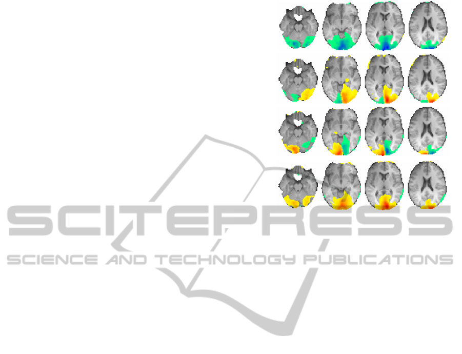
Figure 2 shows average rSPIs derived from the classi-

ﬁcation models in classiﬁcation task I (four classes).

The average prediction accuracy was 0.9229 in terms

of average posterior probability of the correct class.

Figure 2(A) shows the average rSPI across NPAIRS

splits based on the grand average maps s

derived ac-

cording to Procedure I in Section 2.2. The map iden-

tiﬁes that voxels in the visual cortex contribute the

most with relevant information to the classiﬁers. The

average reproducibility of the map across splits was

0.81. Note that the rSPI only contains positive values

since it is based on squared sensitivities. Figure 2(B)

shows average rSPIs that are based on the interclass

contrast (Procedure III in Section 2.2). According to

the map s

le f t|no

a signal increase primarily in the right

visual cortex will increase the posterior probability of

the scans in class (no) being classiﬁed as belonging

to class (left). Figure 1 indicates that this is reason-

able, since the condition (left) is characterized by a

larger signal in the right visual cortex relative to the

(no) condition. Likewise, the map s

le f t|right

indicates

that lowering the signal in the left visual cortex and in-

creasing signal in the right visual cortex will increase

the posterior probability of the scans in class (right)

being classiﬁed as (left). The reproducibility of the

maps in Figure 2 are fairly high ranging from 0.69-

VISUALIZATION OF NONLINEAR CLASSIFICATION MODELS IN NEUROIMAGING - Signed Sensitivity Maps

259

-8

7 22 37

left∣no

0.81

0.80

0.78

0.69

(A)

(B)

left∣right

left∣both

Figure 2: Classiﬁcation task I with a four class classiﬁcation

task. Different brain maps were extracted from the trained

classiﬁer. Panel (A) shows an average rSPI based on the

grand average map (Procedure I in Section 2.2). Panel (B)

shows signed rSPIs based on Procedure III in Section 2.2.

The notation e.g. s

le f t|no

means that the map indicates how

scans in class ’no’ should be changed in order to increase

the posterior probability of class ’left’. The numbers right to

the brain slices denote the reproducibility estimated within

the NPAIRS resampling framework. The rSPIs are thresh-

olded to show the upper 10 percentile of the distribution of

the absolute voxel values, projected onto an average struc-

tural scan of the six subjects included in the analysis. Num-

bers under the slices denote z coordinates in MNI space.

Slices are displayed according to neurological convention.

0.80.

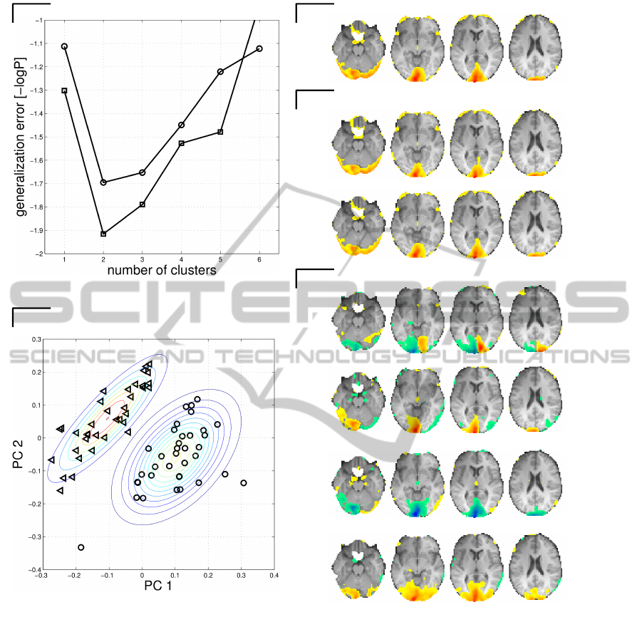
Figure 3(C-E) shows average rSPIs derived from

the classiﬁcation models in classiﬁcation task II (xor-

problem). The average prediction accuracy was

0.905. Figure 3(C) shows the average rSPI across

NPAIRS splits based on the grand average maps s

derived according to Procedure I in Section 2.2. The

maps identify that voxels in the visual cortex that con-

tribute the most relevant information to the classiﬁers.

The average reproducibility of the maps across splits

was 0.81. Note that Figure 3(C) resembles Figure

2(A), which means that the regions identiﬁed as being

relevant to classiﬁcation in tasks I and II are similar.

Figure 3(D) shows average rSPIs based on interclass

contrasts (Procedure III in Section 2.2). Due to the

potential heterogeneity within the classes, the sensi-

tivity maps were based on squared single sensitivities.

Hence, no sign information is present in the maps.

For comparison, we derived signed class speciﬁc

sensitivities directly as in classiﬁcation task I Figure

2(B) (without squaring), and found that the repro-

ducibilities of the maps were reduced to 0.36. This

decrease in reproducibility is presumably due to can-

cellation effects.

Figure 3(E) shows the rSPIs obtained from Pro-

cedure IV in Section 2.2. The ﬁrst and second rows

of Figure 3(E) can be seen as reﬁnements of the ﬁrst

row of Figure 3(D), obtained by dividing the class

{le f t,right} into two clusters. Similarly, the third and

fourth rows of Figure 3(E) are reﬁnements of the sec-

ond row of Figure 3(E).

The clustering process is illustrated in Figure 3(A-

B). Figure 3(B) shows an example of clustering of

observations within class {le f t,right}. In both class

{no,both} and class {le f t,right} we found evidence

of two clusters based on generalization error mea-

sured as the negative likelihood of the Gaussian mix-

ture model (Figure 3(A)). Based on the cluster anal-

ysis we derive two maps for each of the two classes

according to Procedure IV in Section 2.2. By this pro-

cedure we obtained maps with sign information. Fig-

ure 3(E) shows the resulting four rSPI (two for each

class). For example s

{no,both}|{le f t,right},cluster1

denotes

that the sensitivity map is based on the output class

{no,both}, and the sum in eq. (16) is calculated over

the members of class {le f t,right}, where the weight-

ing factor w

is based on the posterior probability

for observations belonging to cluster 1. The repro-

ducibility values of the sensitivity maps are moderate,

ranging from 0.53-0.61. Note that these reproducibil-

ity values are lower than for Procedure III based

on squared single sensitivities (see Figure 3(D)), but

higher than for Procedure III with signed sensitivities

(mean reproducibility 0.36, as stated earlier). To fur-

ther interpret the maps in Figure 3(E) we calculated

the average weight factor w

in eq. (16) for each of the

sub clusters. For the map s

{no,both}|{le f t,right},cluster1

we found that the members of condition (left) had

an average weighting factor of 0.0038 in the sum,

while the members of the condition (right) had an av-

erage weighting factor of 0.9857. Hence, members of

the condition (right) contribute the most to this map.

Likewise, the members of condition (left) contributed

the most to the map s

{no,both}|{le f t,right},cluster2

. For

the map s

{le f t,right}|{no,both},cluster1

we found that the

members of condition (no) had an average weighting

factor of 0.0000 in the sum, while the members of

the condition (both) had an average weighting factor

of 0.9986. Hence, members of the condition (both)

contribute the most to this map. Likewise, the mem-

bers of condition (no) contribute the most to the map

{le f t,right}|{no,both},cluster2

Note the similarity of the maps in the ﬁrst row of

Figure 3(E) (s

{no,both}|{le f t,right},cluster1

, where cluster

1 corresponds to class right, as just explained) and the

second row of Figure 2(B) (s

le f t|right

). Also the fourth

BIOSIGNALS 2012 - International Conference on Bio-inspired Systems and Signal Processing

260

-8

7 22 37

0.81

0.78

0.76

0.53

0.56

0.61

0.56

(C)

(D)

(E)

{no,both}∣{left,right}

{no,both}∣{left,right},cluster 2

{no,both}∣{left,right},cluster 1

{left,right}∣{no,both},cluster 1

{left,right}∣{no,both},cluster 2

(A)

(B)

Figure 3: Classiﬁcation task II. Panel A-B: Structure of single sensitivities. See Procedure IV in Section 2.2 for further

details. Modeling of the data distribution was based on a Gaussian mixture model (GMM). Panel A shows the generalization

error as a function of the number of components (averaged over 10 resampling runs) in the GMM. The generalization error

was calculated by evaluation of the likelihood function of the GMM based on four-fold cross validation performed as a nested

loop within each NPAIRS split half. The circles corresponds to the class s

{no,both}|{le f t,right}

, and the squares corresponds

to the s

{le f t,right}|{no,both}

single sensitivity measures. In both classes we observe evidence for two clusters/components.

Panel B shows contours of the probability densities of a GMM ﬁtted to s

{no,both}|{le f t,right}

sensitivities of a single split

of the data. The triangles corresponds to the observations in condition (left) and the circles corresponds to observations in

the condition (right). Note that this labeling was not ”visible” to the modeling procedure. Panel C-E: Interpretation of the

trained classiﬁer. Different brain maps were extracted from the classiﬁer. Panel (C) shows an average rSPI based on the

grand average sensitivity map (Procedure I in Section 2.2). Panel (D) shows rSPIs based on single class sensitivities. The

notation eg. s

{no,both}|{le f t,right}

means that the map indicates how scans in class {le f t,right} should be changed in order to

increase the posterior probability of class {no,both}. Note that the maps does not contain sign information (Procedure III in

Section 2.2). Panel (E) shows rSPIs based on single class sensitivity, where each class is characterized by two sub-clusters

(Procedure IV in Section 2.2). The numbers right to the brain slices denote the reproducibility estimated within the NPAIRS

resampling framework. The rSPIs are thresholded to show the upper 10 percentile of the distribution of the absolute voxel

values, projected onto an average structural scan of the six subjects included in the analysis. Numbers under the slices denote

z coordinates in MNI space. Slices are displayed according to neurological convention.

VISUALIZATION OF NONLINEAR CLASSIFICATION MODELS IN NEUROIMAGING - Signed Sensitivity Maps

261

row of Figure 3(E) ((s

{le f t,right}|{no,both},cluster2

, where

cluster 2 corresponds to class no) is similar to the ﬁrst

row of Figure 2(B) (s

le f t|both

); and the third row of

Figure 3(E) (s

{le f t,right}|{no,both},cluster1

, where cluster

1 corresponds to class both) is similar to the third row

of Figure 2(C) (s

le f t|both

). The signiﬁcance of these

observations is that Procedure IV has succeeded in

providing similar information when applied to Clas-

siﬁcation Task II (the 2-class xor-problem) as the in-

formation given by Procedure III applied to Classiﬁ-

cation Task I (the 4-class classiﬁcation), even though

the available class labels in Task II are less informa-

tive and the two classes no, both and left, right are

heterogeneous. This suggests that Procedure IV can

provide useful information about the nature of non-

linear classiﬁers when applied to complex, heteroge-

neous classes.

5 CONCLUSIONS

The established probabilistic sensitivity map proce-

dure provides a global summary map of the relative

importance of voxels to a trained classiﬁer (Kjems

et al., 2002). However, no sign information is present

in such a map. In the present work we have pro-

posed a procedure to allow for generation of sum-

mary maps with sign information. Furthermore, we

have proposed a clustering procedure that is applica-

ble in cases where relatively large heterogeneity be-

tween observation exists which may degrade the per-

formance of the model visualization due to cancella-

tion effects.

As a proof of concept, we have illustrated the ap-

proach on a data set from a simple fMRI experiment,

with classes deliberately deﬁned to be heterogeneous.

Our procedure successfully recovered known struc-

ture in the classes. We also found that the maps pro-

duced for this data set are robust, in the sense that

they are reproducible as judged by the NPAIRS re-

sampling framework. We showed that reproducibility

is improved by the new clustering procedure.

Our results suggest that our new method of model

visualization may be useful in visualizing nonlinear

classiﬁers trained on heterogeneous classes. Further

work is needed to compare variations of the method,

in particular different possible choices of the visual-

ization function (see Section 2.2.2), and to validate

the method on a larger variety of real or synthetic data.

ACKNOWLEDGEMENTS

This work is partly supported by the Danish Lundbeck

Foundation through the program www.cimbi.org. The

Simon Spies Foundation is acknowledged for dona-

tion of the Siemens Trio scanner. Kristoffer H. Mad-

sen was supported by the Danish Medical Research

Council (grant no. 09-072163) and the Lundbeck

Foundation (grant no. R48-A4846).

REFERENCES

Baehrens, D., Schroeter, T., Harmeling, S., Kawanab, M.,

Hansen, K., and M

uller, K.-R. (2010). How to ex-

plain individual classiﬁcation decisions. Journal of

Machine Learning Research, 11:1803–1831.

Cox, D. D. and Savoy, R. L. (2003). Functional magnetic

resonance imaging (fMRI) ”brain reading”: detecting

and classifying distributed patterns of fMRI activity in

human visual cortex. NeuroImage 19, pages 261–270.

Davatzikos, C., Ruparel, K., Fan, Y., Shen, D., Acharyya,

M., Loughead, J., Gur, R., and Langleben, D. (2005).

Classifying spatial patterns of brain activity with ma-

chine learning methods: application to lie detection.

NeuroImage, 28(3):663–668.

Friedman, J. H. (1989). Regularized discriminant analysis.

J. Am. Statistical Assoc., 84:165 – 175.

Golland, P., Grimson, W. E. L., Shenton, M. E., and Kikinis,

R. (2005). Detection and analysis of statistical differ-

ences in anatomical shape. Medical Image Analysis,

9:69–86.

Haynes, J. D. and Rees, G. (2006). Decoding mental states

from brain activity in humans. Nature Reviews Neu-

roscience, 7(7):523–534.

Kjems, U., Hansen, L. K., Anderson, J., Frutiger, S., Mu-

ley, S., Sidtis, J., Rottenberg, D., and Strother, S. C.

(2002). The quantitative evaluation of functional neu-

roimaging experiments: mutual information learning

curves. NeuroImage, 15(4):772–786.

LaConte, S., Strother, S., Cherkassky, V., Anderson, J., and

Hu, X. (2005). Support vector machines for temporal

classiﬁcation of block design fMRI data. NeuroImage,

26:317–329.

Lautrup, B., Hansen, L., Law, I., Mørch, N., Svarer, C.,

and Strother, S. (1994). Massive weight sharing: A

cure for extremely ill-posed problems. Proceedings of

the Workshop on Supercomputing in Brain Research:

From Tomography to Neural Networks. World Scien-

tiﬁc, Ulich, Germany, pages 137–148.

Mika, S., R

atsch, G., Sch

olkopf, B., Smola, A., Weston, J.,

and M

uller, K.-R. (1999). Invariant feature extraction

and classiﬁcation in kernel spaces. Advances in Neu-

ral Information Processing Systems, 12:526–532.

Misaki, M., Kim, Y., Bandettini, P., and Kriegeskorte, N.

(2010). Comparison of multivariate classiﬁers and re-

sponse normalizations for pattern-information fMRI.

NeuroImage, 53(1):103–118.

Mørch, N., Hansen, L. K., Strother, S. C., Svarer, C., Rot-

tenberg, D. A., Lautrup, B., Savoy, R., and Paulson,

O. B. (1997). Nonlinear versus Linear Models in

Functional Neuroimaging: Learning Curves and Gen-

eralization Crossover. IPMI ’97: Proceedings of the

BIOSIGNALS 2012 - International Conference on Bio-inspired Systems and Signal Processing

262

15th International Conference on Information Pro-

cessing in Medical Imaging, pages 259–270.

Mour

ao Miranda, J., Bokde, A., Born, C., Hampel, H., and

M (2005). Classifying brain states and determining

the discriminating activation patterns: support vector

machine on functional MRI data. NeuroImage, 28:980

– 995.

O’Toole, A. J., Jiang, F., Abdi, H., P Nard, N., Dunlop, J. P.,

and Parent, M. A. (2007). Theoretical, statistical, and

practical perspectives on pattern-based classiﬁcation

approaches to the analysis of functional neuroimaging

data. Journal of Cognitive Neuroscience, 19:1735–

1752.

Pereira, F., Mitchell, T., and Botvinick, M. (2009). Machine

learning classiﬁers and fMRI: a tutorial overview.

NeuroImage, 45(1):S199–S209.

Rasmussen, P. M., Madsen, K. H., Lund, T. E., and Hansen,

L. K. (2011). Visualization of nonlinear kernel mod-

els in neuroimaging by sensitivity maps. NeuroImage,

55(3):1120 – 1131.

Schmah, T., Yourganov, G., Zemel, R., Hinton, G., Small,

S., and Strother, S. (2010). A Comparison of Classiﬁ-

cation Methods for Longitudinal fMRI Studies. Neu-

ral Computation, 22:2729–2762.

Shawe-Taylor, J. and Cristianini, N. (2004). Kernel methods

for pattern analysis. Cambridge.

Sigurdsson, S., Philipsen, P., Hansen, L., Larsen, J.,

Gniadecka, M., and Wulf, H. (2004). Detection

of skin cancer by classiﬁcation of Raman spec-

tra. IEEE Transactions on Biomedical Engineering,

51(10):1784–1793.

Strother, S., Anderson, J., Hansen, L., Kjems, U., Kustra,

R., Sidtis, J., Frutiger, S., Muley, S., LaConte, S., and

Rottenberg, D. (2002). The quantitative evaluation of

functional neuroimaging experiments: The NPAIRS

data analysis framework. NeuroImage, 15(4):747–

771.

Yourganov, G., Schmah, T., Small, S., PM, R., and Strother,

S. (2010). Functional connectivity metrics during

stroke recovery. Arch Ital Biol., 148(3):259–270.

Zhang, J., Anderson, J. R., Liang, L., Pulapura, S. K.,

Gatewood, L., Rottenberg, D. A., and Strother,

S. C. (2009a). Evaluation and optimization of fMRI

single-subject processing pipelines with NPAIRS and

second-level CVA. Magn Reson Imaging, 27:264–

278.

Zhang, Z., Dai, G., and Jordan, M. I. (2009b). A ﬂexible

and efﬁcient algorithm for regularized ﬁsher discrim-

inant analysis. In ECML PKDD ’09: Proceedings of

the European Conference on Machine Learning and

Knowledge Discovery in Databases, pages 632–647,

Berlin, Heidelberg. Springer-Verlag.

Zurada, J., Malinowski, A., and Cloete, I. (1994). Sensitiv-

ity analysis for minimization of input data dimension

forfeedforward neural network. 1994 IEEE Interna-

tional Symposium on Circuits and Systems, 1994. IS-

CAS’94., 6:447–450.

Zurada, J., Malinowski, A., and Usui, S. (1997). Perturba-

tion method for deleting redundant inputs of percep-

tron networks. Neurocomputing, 14(2):177–193.

APPENDIX

In the following we show how to calculate the deriva-

tive used in eq. (7,8,9). First we calculate the deriva-

tive in eq. (4)

∂z

∂x

∂k

∂x

HB. (17)

We then calculate the derivative of the visualization

function

∂log(p(c|z

))

∂x

∂log(p(z

|c)P(c))

∂x

−

∂log(

∑

p(z

)P(c

))

∂x

−

∂||z

− µ

∂x

∑

p(c

)

∂||z

− µ

∂x

−

∂z

∂x

− µ

) +

∂z

∂x

∑

p(c

)(z

− µ

) =

−

∂z

∂x

− µ

) −

∑

p(c

)(z

− µ

)

−

∂k

∂x

− µ

) −

∑

p(c

)(z

− µ

)

. (18)

For example, for the linear kernel we have

∂k

∂x

= X, (19)

where X holds training observations in the columns.

For the RBF kernel we have

∂k

∂x

= MD

, (20)

where M in a (P × N) matrix that holds the elements

i, j

= x

− x

, with x

referring to the i’th element in

the j’th training example. D

is an (N × N) diagonal

matrix with the elements of k

in the diagonal.

VISUALIZATION OF NONLINEAR CLASSIFICATION MODELS IN NEUROIMAGING - Signed Sensitivity Maps

263