REVERSE PAINTERLY RENDERING

Ying Wang and Masahiro Takatsuka

Vislab, School of IT, University of Sydney, Sydney, Australia

Keywords: Reverse Painterly Rendering (RPR), Painterly Rendering, Image Feature Extraction.

Abstract: Traditional painterly rendering algorithms transform photographic images to their artistic representations

such as paintings or drawings. However, the reverse process of painterly rendering has never been

discussed, which could be useful for studies in heritage and forensic science. This paper presents a novel

reverse painterly rendering algorithm which restores “oil painting-like” images to photo-like images.

Results show that our algorithm can improve the photorealistic appearance of “oil painting-like” images.

1 INTRODUCTION

Previously, many painterly rendering algorithms

were proposed to automatically generate artistic

‘painting-like’ images from photographic images.

However, procedures involved in these algorithms

are usually non-reversible, meaning that original

photographic images cannot be regenerated from

rendered results. However, the reverse process of

painterly rendering can be useful to some

applications such as artwork restoration in heritage

studies, facial reconstruction from sketch in forensic

science. In case where paper based artworks need to

be visualized, reverse painterly rendering can

enhance the realistic appearance of painting images

by transforming them into ‘photograph-like’ images.

This paper mainly focuses on the reverse process of

painterly rendering problem, and aims to develop a

reverse algorithm to restore photographic images

from painterly rendered images with oil painting

effect. To solve reverse painterly rendering (RPR)

problem, 48 image features are extracted, from

which 5 key features are selected. Then an artificial

neural network is trained to predict the 5 key

features of the output (‘photograph-like’ image)

from the input (painterly rendered images with oil

painting effect). Using the selected key features,

signal independent noise which was mainly caused

by additive background texture can be removed and

then we adaptively adjust the colour style and the

smoothness of the contour through our selected 5

key features. Finally, the performance of our

algorithm is measured against ground truth.

The rest of this paper is organized as follows:

section 2 briefly reviews previous works in painterly

rendering; section 3 introduces our proposed reverse

painterly rendering (RPR) algorithm; section 4

presents the results of our algorithm; section 5

discusses the results; finally, section 6 concludes the

paper.

2 RELATED WORKS

Previously, many “forward” painterly rendering

algorithms were proposed. Typically, they take

photographic images as inputs and generate images

with artistic styles. Based on the rendering

techniques, they can be categorized as “stroke-

based” and “example-based” painterly rendering.

In stroke-based painterly rendering, an image is

created by combining an ordered list of strokes

described parametrically by a stroke model

(Hertzmann, 2003). Haeberli was the earliest who

demonstrated an interactive painting application for

simulating painterly brush strokes (Haeberli, 1990).

Although his application does not automate brush

strokes rendering, it demonstrates the earliest idea

on stroke based painterly rendering. Hertzmann

formulated stroke based painterly rendering as an

energy minimization problem (Hertzmann, 2001).

However, solving an energy relaxation problem

remains a computationally expensive task. Although

some stroke based algorithms focus on rendering

specific artistic styles such as impressionist

(Litwinowicz, 1997) and Chinese painting (Xu et al.,

2006); most of them do not explicitly have control

over the rendered styles.

241

Wang Y. and Takatsuka M..

REVERSE PAINTERLY RENDERING.

DOI: 10.5220/0003814802410247

In Proceedings of the International Conference on Computer Graphics Theory and Applications (GRAPP-2012), pages 241-247

ISBN: 978-989-8565-02-0

 2012 SCITEPRESS (Science and Technology Publications, Lda.)

Example-based painterly rendering algorithms

present a new approach for painterly rendering.

Hertzmann et al. present a novel framework called

“image analogy” for transforming photos into

painting-like images by examples (Hertzmann et al.,

2001). In their work, painterly rendering is

formulated as a problem of finding analogy. The

output image is constructed by a block-wised multi-

resolution synthesis. The central idea of this

synthesis technique is to search for the best match

image block from the examples and the input image.

In summary, stroke-based algorithms simulate

the actual painting process. Since brush strokes are

placed one by one on the canvas just as artists do, it

is extremely difficult to derive the reverse process.

Exampled-based painterly rendering algorithms

produce the output by investigating and synthesizing

the pixel level features of examples. However, the

reverse process remains rather difficult because

photographic image details are lost during the

synthesis process. Although various algorithms were

proposed to solve painterly rendering problem, none

of them addressed its reverse process. This is

particularly useful for studies in heritage and

forensic science where photorealistic images of

paintings may be needed. We will introduce reverse

painterly rendering (RPR) algorithm in the next

section.

3 REVERSE PAINTERLY

RENDERING (RPR)

3.1 Problem Formulation

Assume the original photographic image is x(i,j),

and its painted version is y(i,j), the problem of

painterly rendering (particularly with oil painting

effect) can be formulated as:



(

i, j

)

= ∗( ∗((i, j)))+ . (1)

Where n is signal independent noise, which are

caused by adding background textures such as the

texture of canvas to photographic image x. c denotes

a filtering process which incurs signal dependent

noise or distortion to x. For instance, c particularly

causes the distortion of x’s edges and gradient. h is a

2d filter that transforms x’s colour style from

photographic colours to painted colours , * is 2D

convolution.

Therefore, the problem of RPR is to estimate the

original photographic image x through the painterly

rendered image y.

3.2 Solving RPR

3.2.1 Features Extraction

A number of image features are extracted. They can

be categorized as: colour-related, texture-related and

wavelet-related features (Table 1).

Table 1: Extracted image features.

Categories Specific Image Features

Colour- related

Features

Smoothness of colour

Colour palette

Colour saturation

Prevalent colour coverage

Texture-related

Features

Global Gabor filter responses

Local Gabor filter responses

Wavelet-related

Features

First order statistics of first

scale wavelet sub-band

coefficients

In colour-related features, Smoothness of colour

presents the spatial variation of colour in an image

plane. Colour palette accounts for the number of

unique colours in an image. Colour saturation is the

saturation of pixel colours indicated by H channel in

HSV colour space. We extract above three features

using methodology described by (Cutzu et al.,

2005). Prevalent colour coverage presents the

coverage of the most frequently appearing colour in

an image, which was used to distinguish

photographs from graphics on the web in (Athitsos

et al., 1997).

Following the methodology introduced by

(Bianconi and Fernandez, 2007), we extract texture

features using statistics of Gabor filter responses at

five different scales and four different orientations.

Global Gabor filter response is obtained by

averaging Gabor filter responses from all scales and

orientations of a gray scale image. Local Gabor

filter responses are Gabor filter responses from five

different scales (0, 0.2, 0.4, 0.6, 0.8) and four

different orientations (0,













), respectively.

The four first order statistics (mean, variance,

skewness and kurtosis) of wavelet sub-band

coefficients were used in (Lyu and Farid, 2005) and

(Wang and Moulin, 2006) to distinguish computer

generated photorealistic images from real

photographic images. Similarly, we adopt first order

statistics of first scale wavelet sub-band coefficients

as wavelet-related features.

All the features described above are normalized

by the size of the image so that we obtain a score for

each individual feature. RGB colour images are

converted to greyscale images to extract texture and

GRAPP 2012 - International Conference on Computer Graphics Theory and Applications

242

wavelet related features. All the extracted features

form the feature space F. F is a 48 dimensional

vector, and each dimension of F corresponds to an

extracted feature. The notation of F is defined as

follows:

=







……





(2)

Where

: smoothness of colour

: colour palette

: prevalent colour coverage

: global Gabor filter response

: kurtosis and variance of 1

scale

wavelet high frequency (i.e.

horizontal, vertical and diagonal)

components coefficients

: mean, variance, skewness and

kurtosis of 1

scale wavelet sub band

coefficient histograms

: skewness and kurtosis of colour

saturation histogram

: local Gabor filter responses

To testify if above features can identify the

differences between photographic images and “oil

painting-like” images, we build a Support Vector

Machine (SVM) classifier using above features to

distinguish photographic images from “oil painting-

like” images. We first obtain an image dataset

(Martin, 2001) containing 500 photographic images

and then apply “oil painting effect” to the entire

dataset in Photoshop. Totally, 1000 images (500

photographic images and 500 painterly rendered

images) are obtained. Then, we extract features

defined in formula (2) from obtained image pairs.

Finally, we use 700 images for training SVM to

label them as either “photo” or “painting”, and 300

images for test.

The accuracy of the classification is 0.91.

Therefore, we conclude that features defined in

formula (2) are able to characterize the differences

between photographic images and “oil paint-like”

images.

3.2.2 Key Features Selection and Prediction

Among all the obtained 48 image features, we want

to further select the key features that contribute most

to the classification result. We use t-test (Guyon and

Elisseeff, 2003) to assess the significance of each

feature for separating two labelled groups (“photo”

and “painting”). Table 2 shows 10 highest ranked

features.

In Table 2, the top 5 key features are: f

, f

(see formula (2) for definition).

Table 2: List of ranked features by t-test.

10 highest ranked

features

Feature category T-test scores

Colour-related 19.8797

, f

Texture-related 18.2364~

12.9264

, f

Wavelet-related 12.6664~

11.9440

We then use 5 highest ranked features to train the

SVM classifier again. The accuracy of the

classification is 0.82, proving that the 5 highest

ranked features (out of 48 features) are able to

represent the entire feature set.

To reverse an “oil painting-like” image to a

“photo-like” image, we need to predict the above 5

key features of the original photographic image.

Artificial neural network was used for the

prediction. We use the same image dataset to train a

back propagation neural network with key features

of 350 image pairs (i.e. 350 painterly rendered

images as inputs, 350 photographic images as

targets). 150 image pairs are used for test. Table 3

shows Mean Squared Error (MSE) of predicted 5

key features.

Table 3: MSE of predicted key features.

Features f

MSE (×10

-3

) 3.1 6.1 5.5 5.4 5.6

Given an “oil painting-like” image as input, the

output of our RPR algorithm should be an image

whose key features are close to the key features of

the photographic image.

3.2.3 Signal Independent Noise Removal

Based on formula (1), the additive noise n needs to

be removed. The cause of n is primarily from adding

a background texture such as canvas to an image,

therefore n is independent from x. We assume n has

constant variance which can be estimated by feature

: global Gabor filter response. 2D adaptive wiener

filter is used for noise removal. At each pixel point

y(i, j), we calculate the local mean and local

variance of y(i, j) within its neighbourhood, and then

the following formula is applied to reduce the noise:



(

i,j

)

=mean















(

i,j

)

−mean



) .

(3)

Where mean

and var

are local mean and local

variance of pixel point y(i, j) within its

neighbourhood. y

is the result image. var

is the

variance of the signal independent noise estimated

by Global Gabor filter response (feature f

). The

result of applying this filtering to a painterly

REVERSE PAINTERLY RENDERING

243

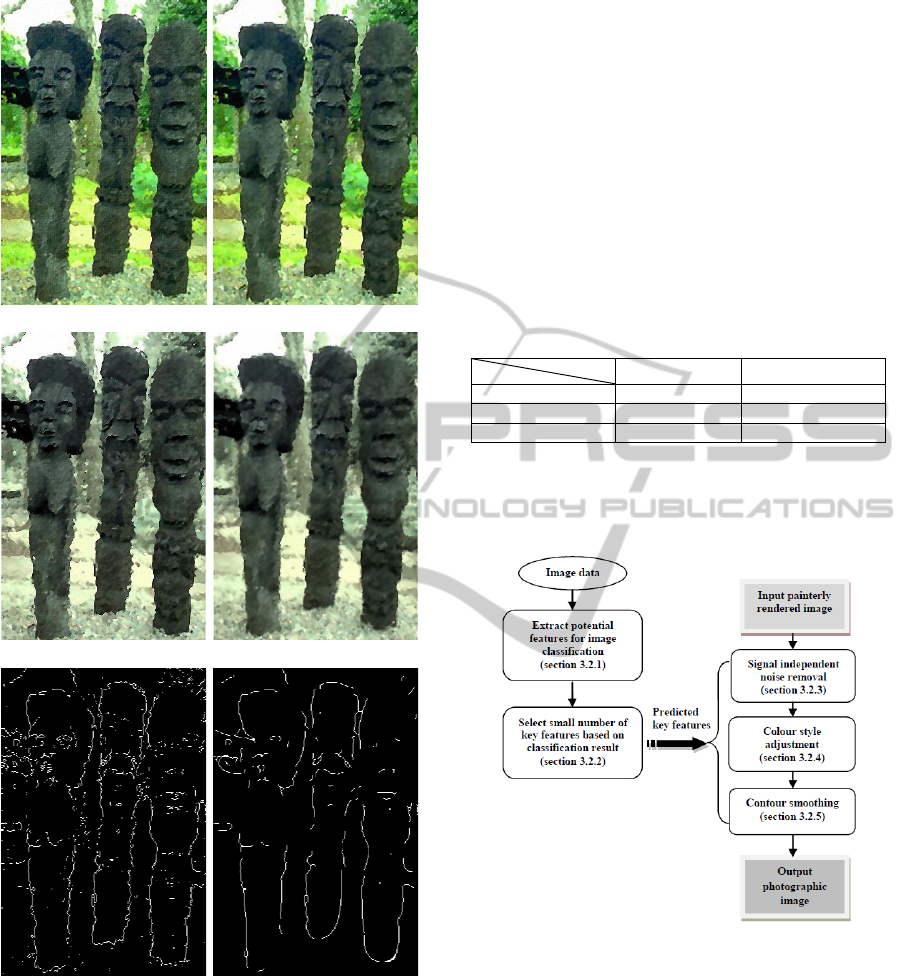
rendered image is shown in Figure 1(b).

3.2.4 Colour Style Adjustment

In formula (1), the effect of 2D colour filtering h

needs to be reversed. To adjust the colour style, we

make use of the highest ranked feature f

: colour

palette. First, we convert the image y

in formula (3)

from RGB to HSV colour space. Then 2D LMS

(Least Mean Square) algorithm is applied to the

saturation channel of the image y

. After the process,

the image is converted back to RGB colour space.

At each iteration,





′

(

i,j

)

=

∑∑

(

i,j

)



(

i,j

)









.

(4)



(

i,j

)

=w

(

i,j

)

+err×



(

i,j

)











.

(5)

err=r×(predicted

–current

).

(6)

Where m and n are the height and width of the

image y

. w is a 2D weight mask used for filtering. r

is a constant that controls the learning rate. This

colour filtering process will run iteratively until error

is less than 0.01. The result of colour style

adjustment is shown in Figure 1(c).

3.2.5 Contour Smoothing

Finally, we need to reduce signal dependent

distortion c in formula (1). From our observation, c

primarily causes the jerkiness of edges and the

uneven changes of colour (i.e. gradient) in an image.

In the feature space, c causes the differences

between painterly rendered images and photographic

images in local Gabor filter responses, i.e. f

, f

and f

. The effect of c can be alleviated by

iteratively smoothing the contour of the image.

Since LUV colour space separate image luminance

from colour, we smooth the image contour in each

channel of LUV colour space. We first extract the

edges of an image. Then we remove small objects

from the edges and smooth the remaining edges

using local regression. For each point on the

remaining edges, we sample its N neighbouring

points on each side and a local regression line is

computed. Then the current point is projected on this

line. The result of smoothed edges is shown in

Figure 1(f).

After we obtain the smoothed edge (e.g. Figure

1(f)), we use it to smooth image contour obtained

from colour style adjustment (e.g. Figure 1(c)). We

first convert the image to LUV colour space. For

each channel, we calculate the gradient towards

horizontal direction and vertical direction. And the

gradient map is the magnitude of the gradient, i.e.

GradientMap =



∇x



+∇y



. (7)

Where ∇x and ∇y are image gradient toward

horizontal and vertical directions.

For each pixel in the image, if it is on both of the

original edges (e.g. Figure 1(e)) and the smoothed

edges (e.g. Figure 1(f)), we leave it unchanged. If it

is on the original edges but not on the smoothed

edges, we change the pixel value to the value of its

nearest neighbouring pixel that has the minimum

gradient indicated by gradient Map. Similarly, if it is

not a on the original edges but on the smoothed

edges, we change the pixel value to the value of its

nearest neighbouring pixel that has the maximum

gradient indicated by gradient Map. We run this

smoothing algorithm iteratively until local Gabor

filter responses (f

, f

and f

) are close to the

predicted values. The final result of applying

contour smoothing is shown in Figure 1(d).

3.2.6 Algorithm

The work flow of RPR algorithm is summarized in a

chart (Figure 2). Our algorithm first extracts

potential features for classifying the image data set

(section 3.2.1).Then based on the classification

result, we select and predict five key features to

control the process of RPR (section 3.2.2). Given the

input painterly rendered image, we first remove the

signal independent noise (section 3.2.3); then adjust

the colour style (section 3.2.4) and smooth the

contour (section 3.2.5) to obtain the restored

photograph-like image.

4 RESULTS

4.1 Experimental Data

To acquire image pairs for our experiment, we

download UC Berkley image segmentation dataset

(Martin, 2001) which contains 500 photographic

images of various subjects. The sizes of these

images are either 481×321 or 321×481. Then we use

Photoshop to apply oil painting effect to the entire

dataset. Eventually, a total number of 1000 images

containing 500 original photographic images and

500 painterly rendered images are obtained.

4.2 Experimental Result

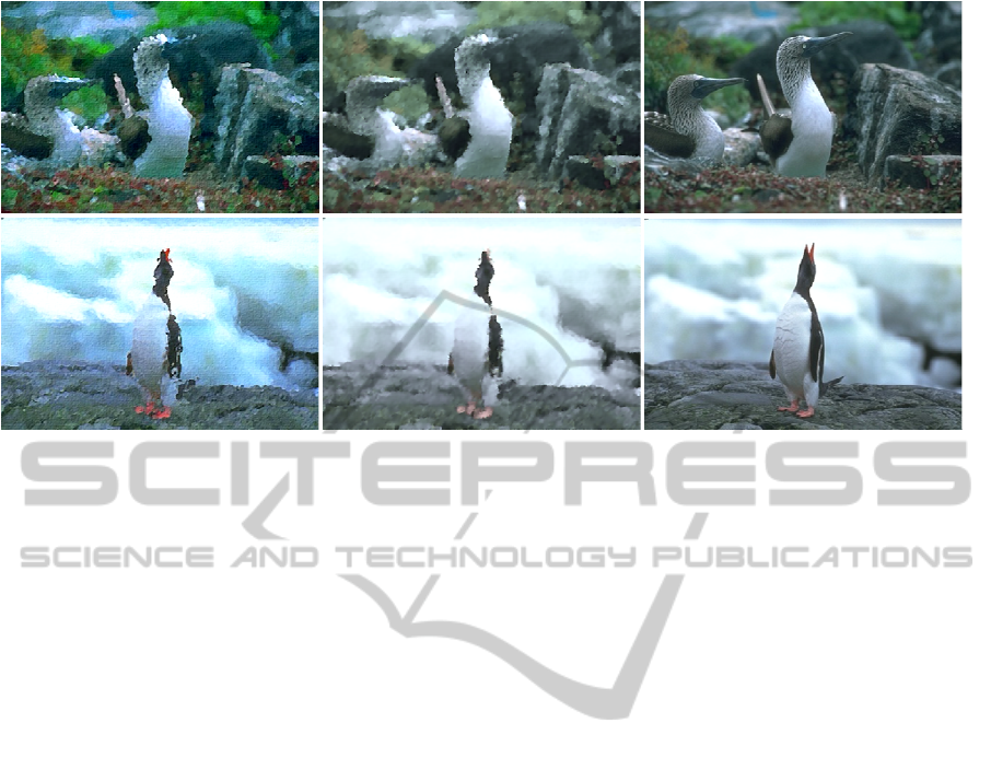
Figure 3 shows our RPR result compared with

ground truth images. In Figure 3, Column A (left) is

GRAPP 2012 - International Conference on Computer Graphics Theory and Applications

244



a. Painterly rendered image. b. After noise removal.

c. After colour filtering. d. After contour smoothing.

e. Original edges. f. Smoothed edges.

Figure 1: Three step process of RPR algorithm.

images with oil painting effect; Column B (middle)

is the photo-like images restored by our RPR

algorithm; Column C (right) is the original photos.

Images of column A are obtained by applying oil

painting effect to column C in Photoshop. Therefore,

column C can be used as ground truth for measuring

the performance of the result.

4.3 Performance

We first compare the absolute image difference

( D

restored-orignal

) between our restored photographic

images and the original photographic images with

the difference ( D

painting-orignal

) between the painterly

rendered images and the original photographic

images. Since LUV colour space separates

luminance from colour, we calculate the average

pixel-wised absolute difference through three

channels in LUV colour space. Table 4 are

restored-orignal

and D

painting-orignal

of images shown in

Figure 3.

Table 4: Comparison of the image differences in Figure 3.

restored-orignal

painting-orignal

row of Figure 3 3.6906 6.4089

row of Figure 3 2.5018 4.2270

Average 3.0962 5.3180

From Table 4, we can see that our algorithm

manages to reduce the pixel-wised image difference

between painterly rendered images and photographic

images.

Figure 2: The workflow of RPR algorithm.

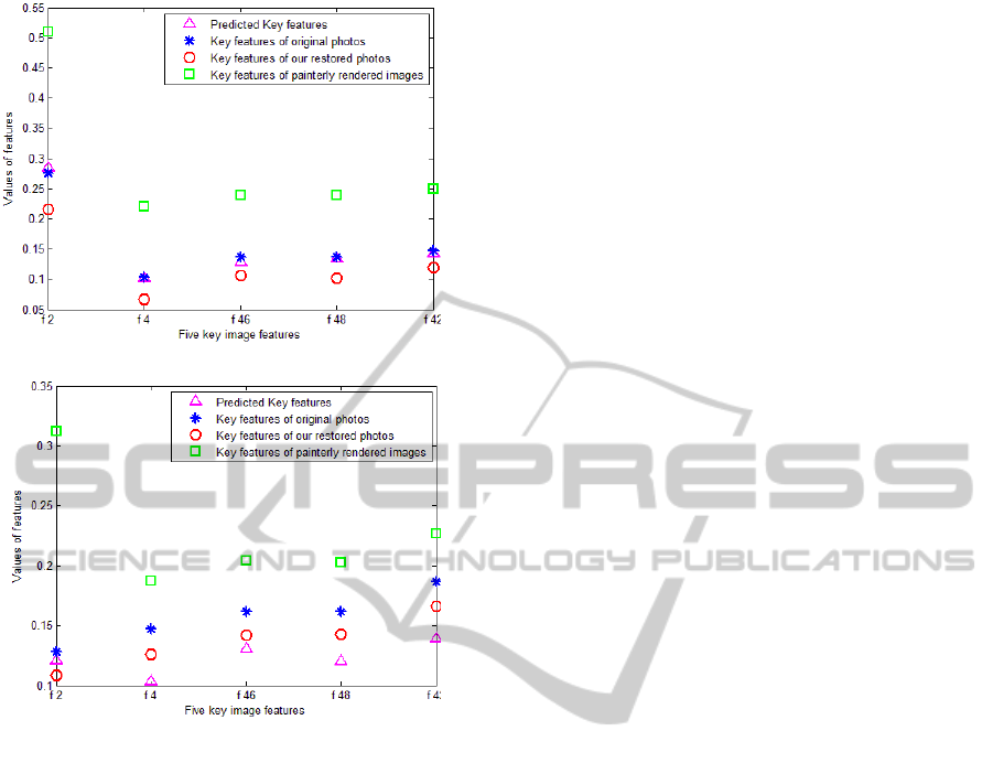
Furthermore, we compared the five key features

, f

) of our experimental result shown

in Figure 3. Figure 4 is the comparison results. To

measure the differences of key features shown in

Figure 4, we can calculate the Euclidean distances

between predicted and original key features, key

features of our restored and original photos, key

features of painterly rendered images and original

photos. In Figure 4, key features of restored

photograph-like images are closer to the original

photographs than “oil painting-like” images. In the

feature space, our algorithm manages to reduce the

REVERSE PAINTERLY RENDERING

245

A. Painterly rendered images. B. Restored photographs by RPR. C. Original photographs.

Figure 3: Results of Reverse Painterly Rendering (RPR).

Euclidean distance between key features of painterly

rendered images and photographic images.

From measuring the pixel-wised image

difference and Euclidean distances of key features,

we can conclude that our RPR algorithm indeed

improves the visual realistic appearance of painterly

rendered images by reducing the pixel-wised

difference and distance of key features from their

original photographic images.

5 DISCUSSION

From the results, we can see that our RPR algorithm

manages to reduce the differences between “oil

painting-like” images and true photographic images.

However, our restored images are still visually

different from photographic images. Especially

when the original photographs have more detailed

regions (such as trees or grass), our algorithm does

not perform very well. This is because important

image details are lost or distorted during the forward

process of painterly rendering. Furthermore, since

the distortion of image edges and gradient in the

process of painterly rendering is still not well

studied, our contour smoothing algorithm remains to

be improved. Additionally, our painterly rendered

images are limited to the “oil painting effect” in

Photoshop; this is because we found the “oil

painting effect” generated by Photoshop is closer to

oil paintings produced by human artists than any

other software such as Irfanview or Paint shop pro.

However, in the future, we would still like to work

on real oil paintings of various styles and

particularly study how contours of objects in oil

paintings are differentiated from photographs.

Meanwhile, image super-resolution and synthesis

technique may be adopted to recover the details of

photographic images.

6 CONCLUSIONS

In this paper, we present a novel RPR algorithm

which can reverse the painterly rendered images

(with oil painting effect) to photograph-like image.

We first formulate the process of painterly rendering

with oil painting effect; then to reverse the process,

we extract important image features through

classifying photographic images from their painterly

rendered images; removing signal independent

noise; adjusting colour style and smoothing

contours. Finally, we measured the performance of

our RPR algorithm. The result shows that our

algorithm is able to improve the photo-realistic

appearance of “oil painting-like” images.

GRAPP 2012 - International Conference on Computer Graphics Theory and Applications

246

a. Key features of images in 1

row of Figure 3.

b. Key features of images in 2

row of Figure 3.

Figure 4: Comparison of five key image features.

REFERENCES

Athitsos, V., Swain, M. J., Frankel, C., 1997.

Distinguishing Photographs and Graphics on the

World Wide Web. IEEE Workshop on Content-Based

Access of Image and Video Libraries, 1997.

Bianconi, F. and Fernandez, A., 2007. Evaluation of the

Effects of Gabor Filter Parameters on Texture

Classification. Pattern Recognition 40 (2007), page

3325-3335.

Cutzu, F., Hammoud, R. and Leykin, A., 2005.

Distinguishing Paintings from Photographs. Comput.

Vis. Image Understanding, vol.100, no. 3, page 249-

273.

Guyon, I. and Elisseeff A., 2003. An Introduction to

Variable and Feature Selection. Journal of Machine

Learning Research 3(2003), page 1157-1182.

Haeberli, P., 1990. Paint by Numbers: abstract image

representations. SIGGRAPH Comput. Graph. page

207-214.

Hertzmann, A., 2001. Paint by Relaxation. Proceedings of

Computer Graphics International (CG1). page. 47-54.

Hertzmann, A., Jacobs, C. E., Oliver, N., Curless, B. and

Salesin, D. H., 2001. Image Analogies. Proceedings of

the 28

annual conference and computer graphics and

iteractive techniques.

Hertzmann, A., 2003. Tutorial: A Survey of Stroke-Based

Rendering. IEEE Comput. Graph. Appl., vol.23, no.4,

2003, page 70-81.

Litwinowicz, P., 1997. Processing Images and Video for

an Impressionist Effect. Proceedings of the 24th

annual conference on computer graphics and

interactive techniques. page 407-414, ACM

Press/Addison-Wesley Publishing Co.

Lyu, S., Farid, H., 2005. How realistic is photorealistic?

IEEE Transactions on Signal Processing, vol.53, no.2,

page 845- 850.

Martin, D., Fowlkes, C., Tal, D., Malik, J., 2001. A

Database of Human Segmented Natural Images and its

Application to Evaluating Segmentation Algorithms

and Measuring Ecological Statistics. Proceedings of

the 8

International Conference on Computer Vision

(ICCV).

Wang Y., Moulin, P., 2006. On Discrimination Between

Photorealistic and Photographic Images. Proceedings

of 2006 IEEE International Conference on Acoustics,

Speech and Signal Processing.

Xu, S., Xu, Y., Kang, S. B., Salesin, D. H., Pan, Y., and

Shum, H.-Y. 2006. Animating Chinese Paintings

Through Stroke-based Decomposition. ACM Trans.

Graph. vol.25, no. 2, page 239–267.

REVERSE PAINTERLY RENDERING

247