SHADOW AND SPECULAR REMOVAL BY PHOTOMETRIC

LINEARIZATION BASED ON PCA WITH OUTLIER EXCLUSION

Takahiro Mori

, Shinsaku Hiura

and Kosuke Sato

Graduate School of Engineering Sciences, Osaka University, 1-3 Machikaneyama, Toyonaka, 560-8531 Osaka, Japan

Graduate School of Information Sciences, Hiroshima City University, 3-4-1 Ozukahigashi, Asaminamiku, 731-3194

Hiroshima, Japan

Keywords:

Photometric Linearization, Reﬂection Components, Shadow Removal.

Abstract:

The photometric linearization method converts real images, including various photometric components such

as diffuse reﬂection, specular reﬂection, attached and cast shadow, into images with diffuse reﬂection compo-

nents only, which satisﬁes the Lambertian law. The conventional method(Mukaigawa et al., 2007) based on

a random sampling framework successfully achieves the task; however, it contains two problems. The ﬁrst is

that the three basis images selected from the input images by the user seriously affect the linearization result

quality. The other is that it takes a long time to process the enormous number of random samples needed to

ﬁnd the correct answer probabilistically. We therefore propose a novel algorithm using the PCA (principal

component analysis) method with outlier exclusion. We used knowledge of photometric phenomena for the

outlier detection and the experiments show that the method provides fast and precise linearization results.

1 INTRODUCTION

Most photometric analysis methods assume that the

input images follow the Lambertian law. It is there-

fore important to generate images with only diffuse

reﬂections from the input images with other photo-

metric components, such as specular reﬂections and

shadows.

Several methods have already been proposed

for separation of photometric components. The

dichromatic reﬂection model(Shafer, 1985) is often

used(Klinker et al., 1988; Sato and Ikeuchi, 1994;

Sato et al., 1997) for the separation. If the colors of

the objects are quite different from the color of the

light source, the model is very effective. However,

if the two colors are similar, the separation becomes

unstable. This method is of course not applicable for

monochromatic images.

The polarization is also useful for the separation

process. Wolff and Boult(Wolff and Boult, 1991) pro-

posed a method to separate specular reﬂections by

analyzing the reﬂected polarization, while Nayar et

al.(Nayar et al., 1993) used combined color and po-

larization clues to separate the specular reﬂections.

These methods, however, have a common restriction

in that they cannot handle shadows. The geometry of

the scene is useful for the analysis of specular reﬂec-

tions and shadows. Ikeuchi and Sato(Ikeuchi and

Sato, 1991) proposed a method to classify photomet-

ric components based on the range and brightness of

the images. A shadowed area can be distinguished us-

ing the shape of the object, but it is not easy to mea-

sure the shape of the scene even in the occluded areas.

However, there are some methods that use the

characteristics of diffuse reﬂection, which lies in a lin-

ear subspace. Shashua(Shashua, 1992) showed that

an image illuminated from any lighting direction can

be expressed by a linear combination of three ba-

sis images taken from different lighting directions,

and assuming a Lambertian surface and a parallel

ray. This means that an image can be perfectly ex-

pressed in a 3D subspace. Belhumeur and Krieg-

man(Belhumeur and Kriegman, 1996) showed that an

image can be expressed using the illumination cone

model, even if the image includes attached shadows.

In the illumination cone, the images are expressed by

using a linear combination of extreme rays. Georghi-

ades et al.(Georghiades et al., 2001) extended the illu-

mination cone model so that cast shadows can also be

expressed using shape reconstruction. Although any

photometric components can ideally be expressed us-

ing the illumination cone, large numbers of images

corresponding to the extreme rays are necessary.

Based on Shashua’s framework, Mukaigawa et

221

Mori T., Hiura S. and Sato K..

SHADOW AND SPECULAR REMOVAL BY PHOTOMETRIC LINEARIZATION BASED ON PCA WITH OUTLIER EXCLUSION.

DOI: 10.5220/0003817202210229

In Proceedings of the International Conference on Computer Vision Theory and Applications (VISAPP-2012), pages 221-229

ISBN: 978-989-8565-03-7

 2012 SCITEPRESS (Science and Technology Publications, Lda.)

al.(Mukaigawa et al., 2007; Mukaigawa et al., 2001)

proposed a method to convert real images into linear

images with diffuse components using only the ran-

dom sample consensus algorithm. The method can

also classify each pixel into diffuse, specular, attached

shadow and cast shadow areas. However, because

their method starts from three manually selected in-

put images, the result depends heavily on the im-

age selection. Their algorithm also takes a very long

time to ﬁnd an adequate combination of diffuse pix-

els from an enormous set of random samples. There-

fore, in this paper, we propose a novel algorithm us-

ing the PCA (principal component analysis) method

with outlier exclusion. This method automatically

generates basis images, and the deterministic algo-

rithm guarantees much a shorter execution time. The

outliers are distinguished by using the knowledge of

photometric phenomena, and the results show that

out algorithm provides better results than those using

RANSAC-based outlier exclusion.

2 CLASSIFYING REFLECTION

USING PHOTOMETRIC

LINEARIZATION

From the viewpoint of illumination and reﬂection

phenomena, each pixel on the input image is classi-

ﬁed into several areas, as shown in Fig.1. Accord-

ing to the dichromatic reﬂection model(Shafer, 1985)

shown in Fig.2, reﬂection consists of diffuse and spec-

ular reﬂections. While the observed intensity caused

by diffuse reﬂection is independent of the viewing di-

rection, specular reﬂection is only observed from a

narrow range close to the mirror direction of the inci-

dent light. Shadows are also classiﬁed into attached

shadows and cast shadows(Shashua, 1992). If the an-

gle between the surface normal and the light direction

is larger than a right angle, the intensity of the sur-

face is zero and is called attached shadow. If there

is an object between the light source and the surface,

the incoming light is occluded by the object. This is

called cast shadow.

In the following, we discuss the reﬂection phe-

nomena using a linear model of diffuse reﬂection.

2.1 Classiﬁcation of Reﬂections

The Lambertian model is a most basic reﬂection

model of a matte surface, such as plaster. The inten-

sity of the surface is represented as

i = n · s (1)

Diffuse reflection

Specular reflection

Cast shadow

Attached shadow

Figure 1: Illumination and reﬂection phenomena.

Reflection

Diffuse Specular

Figure 2: Dichromatic reﬂection model.

where n denotes the surface property vector, which is

a product of a unit normal vector and the diffuse re-

ﬂectance. Similarly, s represents the lighting property

vector, which is a product of a unit vector towards the

lighting direction and the brightness of the light.

In Eq.(1), if the angle between n and s is greater

than 90

◦

, the intensity i becomes negative, but, of

course, there cannot be a negative power of light. In

this case, the area on the object is observed as be-

ing attached shadow, and the intensity becomes zero

instead of the negative value. To deal with the at-

tached shadows as well as the diffuse reﬂections, the

following equation is commonly used(Belhumeur and

Kriegman, 1996).

i = max (n · s, 0) (2)

In contrast, as shown in Fig. 1, the angle between

n and s is smaller than 90

◦

in the area of a cast shadow.

If there is no inter-reﬂection, the intensities of both

shadowed areas are zero, and we can distinguish be-

tween the two shadow phenomena by using the sign

of n · s if we know the surface normal and the lighting

direction.

As shown in Fig. 2, the intensity of the specu-

lar reﬂection is an additional component to the dif-

fuse reﬂection. Therefore, the intensity at the specu-

lar reﬂection is always greater than the value calcu-

lated with the Lambertian model. To summarize, we

can distinguish the illumination and reﬂection com-

ponents using the following chart.











Diffuse i = n · s

Specular i > n · s

Attached shadow i = 0 ∩ n · s ≤ 0

Cast shadow i = 0 ∩ n · s > 0

(3)

VISAPP 2012 - International Conference on Computer Vision Theory and Applications

222

2.2 Photometric Linearization

Shashua(Shashua, 1992) showed that if a paral-

lel ray is assumed, an image with N pixels I

(

(k,1)

(k,2)

··· i

(k,N)

)

of a diffuse object under

any lighting direction can be expressed using a lin-

ear combination of three basis images, (

, and

)

taken using different lighting directions;

= c

+ c

(4)

Here, let C

(

)

be a set of coefﬁcients

of the image I

However, real images do not always satisfy Eq.(4),

because specular reﬂections and shadows are com-

monly observed. Therefore, in this paper, we dis-

cuss the conversion of real images into linear images

which include diffuse reﬂection components only.

This conversion process is called photometric lin-

earization and the converted images are called lin-

earized images. Because linearized images should

satisfy Eq.(4), all M input images could be expressed

by using linear combination of the three basis im-

ages(Shashua, 1992) as

(

·· · I

)

(

)(

·· · C

)

(5)

where i

(k,p)

= i

(k,p)

at the pixel of diffuse reﬂec-

tion. In other words, i

(k,p)

= n

· s

is satisﬁed in lin-

earized images, and we can lead relationships such

that a set of basis images B =

(

)

and a set

of coefﬁcients C =

(

·· · C

)

can be rep-

resented as B =

(

·· · n

)

· Σ and C =

−1

(

·· · s

)

respectively, using the com-

mon 3 × 3 matrix Σ.

2.3 Classiﬁcation using Linearized

Images

As described above, each pixel of the input images

can be classiﬁed into areas of diffuse reﬂection, spec-

ular reﬂection, attached shadow and cast shadow us-

ing the surface normal n and the lighting direction

s. Fortunately, we only use the product of these vec-

tors n · s, and we can also classify them by compar-

ing the pixel values of the input and linearized im-

ages, i

(k,p)

and i

(k,p)

respectively. The classiﬁcation

does not need any additional information, such as 3D

shapes, lighting directions, or color information.

In reality, captured images are affected by various

types of noise. For example, imaging devices produce

a dark current even if the intensity of the scene is zero.

Also, the pixel intensity values are not perfectly linear

Figure 3: Criterion for photometric classiﬁcation.

Figure 4: Specular lobe arise around specular peak.

in actual sensors, and so we often model these noises

sources with additive and multiplicative noise models.

As shown in Figure 3, we classify each pixel with

the following criteria.











Specular R. i

(k,p)

> i

(k,p)

∗ T

∩ i

(k,p)

> i

(k,p)

+ T

Attached S. i

(k,p)

< T

∩ i

(k,p)

≤ 0

Cast S. i

(k,p)

< T

∩ i

(k,p)

> 0

Diffuse R. otherwise

(6)

The thresholds T

and T

shown in Fig.3 are used

to check the equality of i

(k,p)

and i

(k,p)

with certain

multiplicative and additive noises. The t hreshold T

used to distinguish shadows. These thresholds can be

determined through experiments with real images. In

the linearization algorithm described below, we grad-

ually decrease these thresholds to exclude the outliers

properly.

2.4 Handling Specular Lobe

As mentioned in section2.1, the intensity observed at

specular reﬂection points is greater than that at the

points with diffuse reﬂection only. However, in real-

ity, the difference is not always sufﬁciently large, and

the thresholds T

and T

against noise will improp-

erly include specular reﬂections to the inliers. More

speciﬁcally, this phenomenon is commonly observed

at specular lobes. As shown in Fig.4, specular lobes

SHADOW AND SPECULAR REMOVAL BY PHOTOMETRIC LINEARIZATION BASED ON PCA WITH OUTLIER

EXCLUSION

223

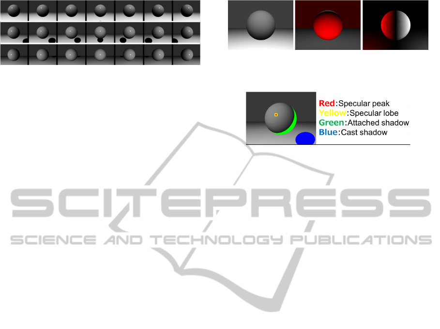
Figure 5: Input images.

surround the specular peaks, so we use spatial infor-

mation to exclude such areas. While the lineariza-

tion method using PCA described in the next section

does not use the information about the neighboring

relationships between pixels, we can exclude the er-

roneous area by increasing the area of the specular

peaks by using the dilation operation. It is there-

fore important not only to exclude outliers during lin-

earization, but also to use classiﬁcation of optical phe-

nomena to expand the specular reﬂection area only.

3 PHOTOMETRIC

LINEARIZATION USING PCA

In this section, we present our linearization algorithm

derived from principal component analysis (PCA).

More speciﬁcally, we combine an outlier exclusion

process based on the classiﬁcation of photometric

phenomena with repetitive PCA.

3.1 Algorithm

The following is the process for our linearization al-

gorithm.

(A) Initialize.

For the photometric linearization, multiple images

I =

(

·· · I

)

, M > 3 as shown in Fig.5

are taken using different lighting directions. While

taking these images, the camera and the target ob-

jects should be ﬁxed, and the information about the

3D shape, the lighting direction and the surface re-

ﬂectance is not necessary. As an initialization, the

input images are copied to the buffer of the inlier im-

ages, I

(

·· · I

)

(B) Calculate Three Basis Images using PCA.

In the conventional method(Mukaigawa et al.,

2007), three manually selected images are converted

into linearized images using the RANSAC algo-

rithm(Fischler and Bolles, 1981). However, as dis-

cussed earlier, this method has a problem in that the

quality of the result depends heavily on the image se-

lection. In contrast, we use all images to calculate the

Figure 6: Three basis images (red color represents negative

value).

Figure 7: Classiﬁcation of photometric components.

linearized image using PCA. More speciﬁcally, we

calculate the 1st, 2nd, and 3rd principal components

B =

(

)

of the matrix I

by analyzing the

eigenvectors of the covariance matrix I

without

subtracting the mean of the input images. Because the

principal components are orthogonal to each other,

we can obtain linearly independent basis images as

shown in Fig.6, where negative values are shown in

red.

The coefﬁcients of the linear combination C are

determined by minimizing the root mean square er-

rors between the input and linearized images as

C = B

(7)

because B is the orthonormal basis and B

B = I. The

linearized images are then calculated by using the ba-

sis images and coefﬁcients,

= B · C (8)

(D) Classiﬁcation of Photometric Components.

As described in section 2.3, each pixel of each

input image is classiﬁed into four photometric com-

ponents, diffuse, specular peak, attached shadow and

cast shadow, by comparing the pixel values of the in-

put image i

(k,p)

and the linearized image i

(k,p)

based

on the photometric classiﬁcation criterion Eq.(6), as

shown in Fig.3.

(E) Extension to Specular Lobe Area.

As shown in Fig.4, specular lobes arise around

specular peaks. Therefore, pixels around the specu-

lar peak area are classiﬁed as outliers by the specular

lobe. Fig.7 shows an example of classiﬁcation for a

scene with a sphere.

VISAPP 2012 - International Conference on Computer Vision Theory and Applications

224

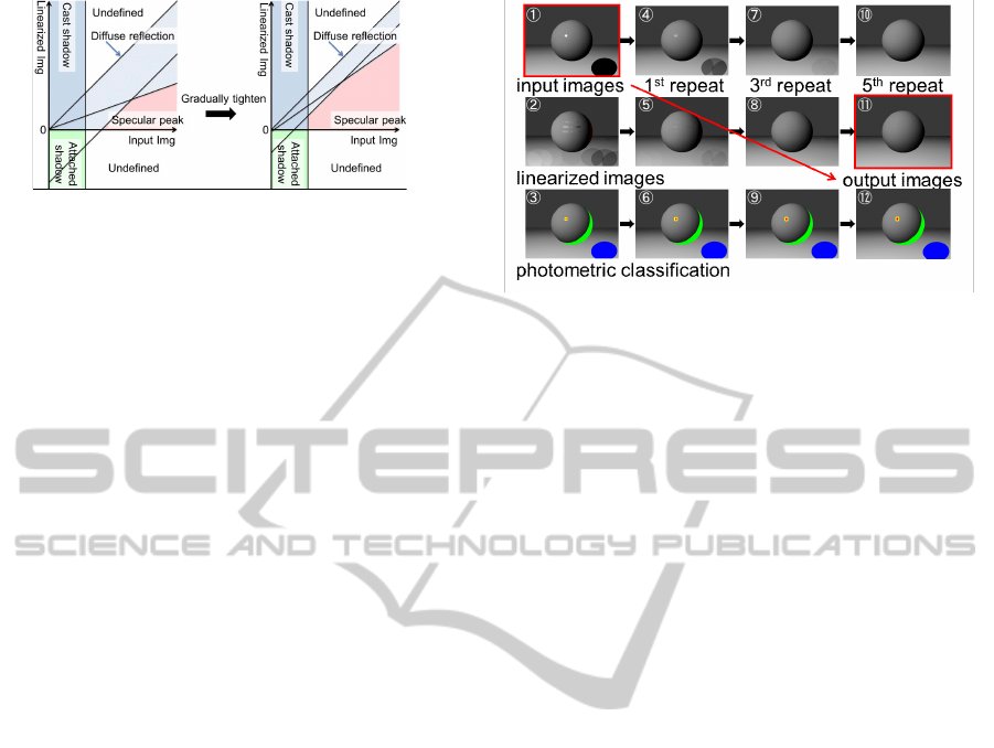
Figure 8: Tightening thresholds with each iteration.

(F) Pixel Value Replacement. Pixels affected by

nonlinear illumination and reﬂection phenomena

should be excluded as outliers for the next iteration

of the PCA calculation,











(k,p)

= i

(k,p)

pixel of diffuse reﬂection

(k,p)

= i

(k,p)

pixel of specular reﬂection,

specular lobe,

attached and cast shadows

(9)

(G) Tighten Thresholds and Iterate.

The algorithm starts from very loose thresholds to

exclude the explicit outliers only. If such evident out-

liers are removed, the result of the next calculation

becomes closer to the correct answer. Therefore, at

this stage, thresholds T

and T

are slightly tightened

towards the values determined for the sensor’s noise

level, as shown in Fig.8. Then, the process sequence

from (B) to (G) is repeated until the thresholds reach

the predetermined minimum values.

3.2 Example

Here, we show an example of each step of the lin-

earization process for the input image shown in Fig.5.

In Fig.9, 1

⃝

shows one of the input images. Because

the initial image contains nonlinear components, the

linearized images calculated by step (C) contain ar-

tifacts, as shown in 2

⃝

. By using the classiﬁcation

result shown in 3

⃝

, the pixel values at the outlier pix-

els of image 1

⃝

are replaced by a linearized image

⃝

in step (F), and the next input image 4

⃝

are gen-

erated. Here, the pixel intensities in the specular and

cast shadow areas are relaxed, so the next linearized

result 5

⃝

is better than the result calculated using the

raw input images. The processes are repeated with

tighter thresholds, and ﬁnally we obtain a clear lin-

earized image

⃝

and correct classiﬁcation results

⃝

4 EXPERIMENTS

In this section, we show several experimental results.

Figure 9: Example of the process of linearization by replac-

ing outliers.

Computationally generated images are used for the

quantitative evaluation because we can render the im-

ages without specular reﬂection and shadows as the

ground truth. Results using real images show the ro-

bustness and feasibility of our method for the actual

task.

4.1 Evaluation using Synthetic Images

First, we evaluated our proposed method by compar-

ison with the conventional method(Mukaigawa et al.,

2007) using synthetic images. The input images were

generated by POV-Ray ray-tracing rendering soft-

ware.

(A) Simple Convex Object.

The scene contains a sphere on a ﬂoor as shown in

Fig.5. In some images, the cast shadow of the sphere

is observed in the image on the ﬂoor. Twenty-one im-

ages were generated, using a different lighting direc-

tion for each image.

Fig.10(a) shows three manually selected images

to be converted as basis images using the conven-

tional method. As described above, the conven-

tional method requires manual selection, which heav-

ily affects the result. The selection shown in the

ﬁgure is one of the adequate selections. Fig.10(b)

shows the ground truths without specular reﬂection

and shadows, corresponding to the three selected im-

ages. While we obtain linearized images for all input

images in the ﬁnal result, we will show these three

images in the paper for comparison purposes.

The result of linearization by the conventional

method are shown in Fig.10(c), with a corresponding

error map (Fig.10(d)). Because the algorithm based

on random sampling, the result shows some noise

caused by the probabilistic ﬂuctuation.

Unlike the conventional method, our algorithm

does not require manual selection. Fig.10(e) shows

the three basis images B =

(

)

where the red

SHADOW AND SPECULAR REMOVAL BY PHOTOMETRIC LINEARIZATION BASED ON PCA WITH OUTLIER

EXCLUSION

225

color indicates negative values. Using these basis im-

ages, we can linearize any input images. Fig.10(f)

shows the results of the linearization of the three in-

put images corresponding to the manually selected

images for the conventional method. The colored er-

ror map shown in Fig.10(g) shows fewer errors when

compared to that of the conventional method. A quan-

titative evaluation is shown in Table 1.

As described above, our method has the other ad-

vantage of fast calculation time. As shown in Table 2,

our method is more than 100 times faster than the con-

ventional method. This is because the conventional

method uses the RANSAC(Fischler and Bolles, 1981)

algorithm to remove the non-Lambertian components

and runs an enormous number of iterative calcula-

tions. If the number of iterations is limited, the result

is degraded.

Table 1: Quantitative evaluation of the result.

Mean error Variance Max. error

Conventional 2.420 2.688 22

Proposed 0.831 1.933 16

Table 2: Comparison of the calculation time.

Calculation time[s]

Conventional 3.930 × 10

Proposed 1.424 × 10

Fig.10(h) shows the classiﬁcation results using the

proposed method. In this ﬁgure, the red, yellow, green

and blue pixels correspond to the specular peaks,

specular lobes, attached shadows and cast shadows

respectively. It is evident that the classiﬁcation has

been performed correctly.

(B) Complex Shaped Object.

We then show the results for the complex shaped

object. The object shape is that of a Stanford bunny,

as shown in Fig.11. Twenty-ﬁve images were gener-

ated, using a different lighting direction for each im-

age.

In Fig.12, we show the results of the conventional

and proposed methods in the same order as Fig.10.

In this case, the conventional method fails. Fig.12(c)

shows that the results contain the remaining specu-

lar areas and noisy values, and the error map shown

in Fig.12(d) also indicates erroneous results. In con-

trast, the proposed method offers adequate results, as

shown in Fig.12(f), which are close in appearance to

the ground truths shown in Fig.12(b). The error map

shown in Fig.12(g) also shows fewer noise compared

to that of the conventional method. Table 3 also indi-

cates a clear difference between the conventional and

(a) Images to be linearized by conventional method.

(b) Ground truths.

(d) Error map of conventional method.

(e) Three basis images generated by proposed method.

(f) Linearized by proposed method.

(g) Error map of proposed method.

(h) Classiﬁed by proposed method.

Figure 10: Linearization of synthetic convex object.

proposed methods. The classiﬁcation results from our

method shown in Fig.12(h) also show that our results

are correct. The calculation time shown in Table4

shows similar differences to the case of the sphere

scene.

VISAPP 2012 - International Conference on Computer Vision Theory and Applications

226

Figure 11: Input images.

Table 3: Numerical evaluation of the linearization result.

Mean error Variance Max. error

Conventional 9.634 410.740 255

Proposed 3.716 28.107 151

Table 4: Comparison of the calculation time.

Calculation time[s]

Conventional 5.132 × 10

Proposed 1.488 × 10

4.2 Evaluation using Real Images

In this section we use real images taken with a cam-

era. The scene contains a pot, as shown in Fig.13.

Twenty-four images were captured, using a different

lighting direction for each one.

Fig.14(a) shows the three input images se-

lected for linearization by the conventional method.

Fig.14(c) shows the linearization result generated

by the conventional method, while Fig.14(d) shows

the linearization result generated by the proposed

method. Both results are similar, but, we can see some

noisy ﬂuctuations on the results from the conventional

method. In contrast, the proposed method provides

smooth images without specular reﬂections. Figure

14(e) shows that our algorithm properly classiﬁes the

phenomena observed on the object. The proposed

method also has the advantage of being much faster

than the conventional method as shown in Table5.

Table 5: Comparison of the calculation time.

Calculation time[s]

Conventional 8.028 × 10

Proposed 1.675 × 10

(a) Images to be linearized by conventional method.

(b) Ground truth.

(d) Error map of conventional method.

(e) Three basis images generated by proposed method.

(f) Linearized by proposed method.

(g) Error map of proposed method.

(h) Classiﬁed by proposed method.

Figure 12: Linearization of complex shaped object.

SHADOW AND SPECULAR REMOVAL BY PHOTOMETRIC LINEARIZATION BASED ON PCA WITH OUTLIER

EXCLUSION

227

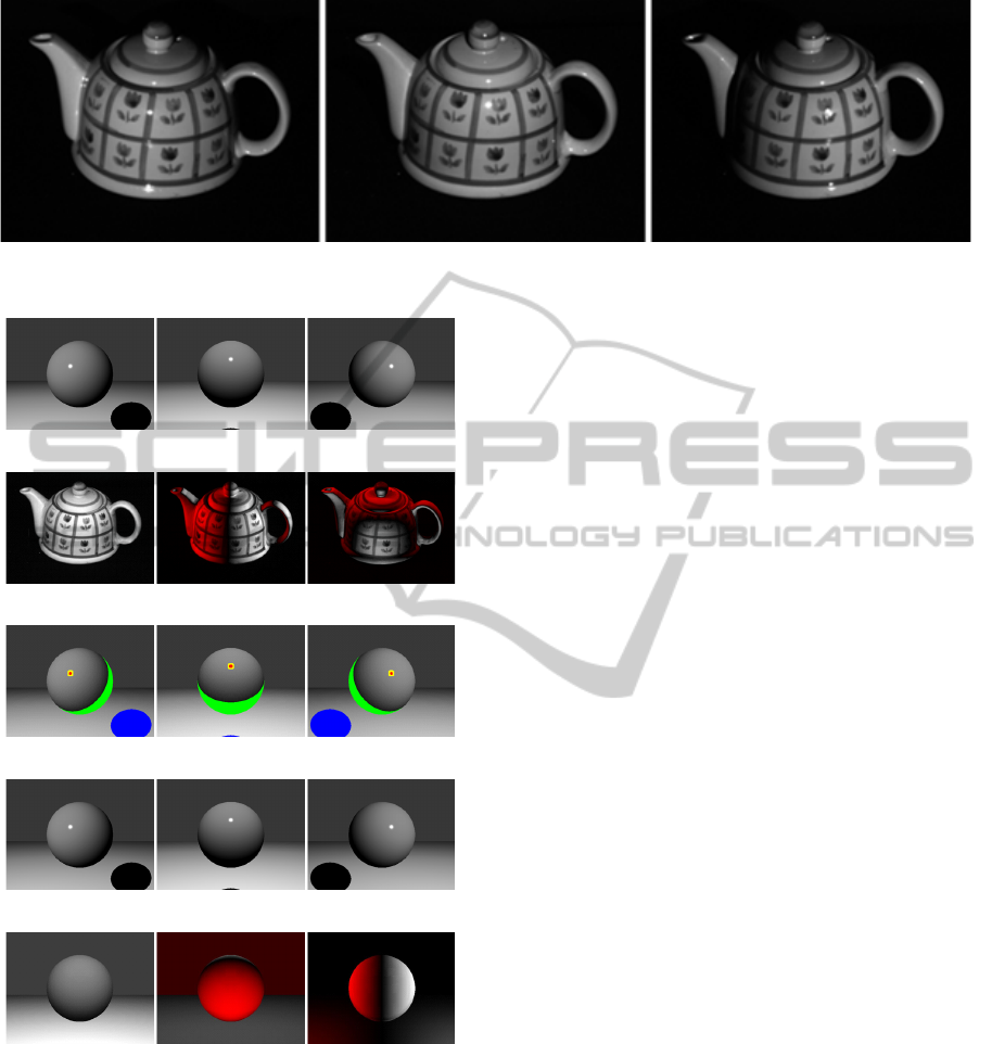
Figure 13: Input images.

(a) Images to be linearized by conventional method.

(b) Three basis images generated by proposed method.

(d) Linearized by proposed method.

(e) Classiﬁed by proposed method.

Figure 14: Linearization of real images.

5 CONCLUSIONS

We focused on the approach of the conventional

photometric linearization method(Mukaigawa et al.,

2007), which selects three basis images from real im-

ages, including not only diffuse reﬂections but also

specular reﬂections and shadows. The conversion ac-

curacy thus becomes unstable and is seriously inﬂu-

enced by the selection of the three basis images, and it

also takes a long time to remove the non-Lambertian

components, e.g. the specular reﬂections and shad-

ows. We therefore proposed a novel pixel value re-

placement algorithm using photometric classiﬁcation,

which enables us to uniquely generate three ideal ba-

sis images, including only diffuse reﬂections from

real images, and enables us to generate accurate ideal

images stably and quickly. We then conﬁrmed the ef-

fectiveness of the proposed method experimentally.

ACKNOWLEDGEMENTS

The authors are grateful to Prof. Mukaigawa and Mr.

Ishii for providing their source codes and real images

presented in their paper (Mukaigawa et al,, 2007) for

our comparisons shown in Section 4. This work was

partially supported by Grant-in-Aid for Scientiﬁc Re-

search (B:21300067) and Grant-in-Aid for Scientiﬁc

Research on Innovative Areas (22135003).

REFERENCES

Belhumeur, P. and Kriegman, D. (1996). What is the set

of images of an object under all possible lighting con-

ditions? In cvpr, page 270. Published by the IEEE

Computer Society.

Fischler, M. and Bolles, R. (1981). Random sample con-

sensus: a paradigm for model ﬁtting with applications

to image analysis and automated cartography. Com-

munications of the ACM, 24(6):381–395.

Georghiades, A., Belhumeur, P., and Kriegman, D. (2001).

From few to many: Illumination cone models for face

recognition under variable lighting and pose. Pat-

tern Analysis and Machine Intelligence, IEEE Trans-

actions on, 23(6):643–660.

Ikeuchi, K. and Sato, K. (1991). Determining reﬂectance

properties of an object using range and brightness im-

ages. IEEE Transactions on Pattern Analysis and Ma-

chine Intelligence, pages 1139–1153.

VISAPP 2012 - International Conference on Computer Vision Theory and Applications

228

Klinker, G., Shafer, S., and Kanade, T. (1988). The mea-

surement of highlights in color images. International

Journal of Computer Vision, 2(1):7–32.

Mukaigawa, Y., Ishii, Y., and Shakunaga, T. (2007). Anal-

ysis of photometric factors based on photometric lin-

earization. JOSA A, 24(10):3326–3334.

Mukaigawa, Y., Miyaki, H., Mihashi, S., and Shakunaga, T.

(2001). Photometric image-based rendering for image

generation in arbitrary illumination. In Computer Vi-

sion, 2001. ICCV 2001. Proceedings. Eighth IEEE In-

ternational Conference on, volume 2, pages 652–659.

IEEE.

Nayar, S., Fang, X., and Boult, T. (1993). Removal of

specularities using color and polarization. In Com-

puter Vision and Pattern Recognition, 1993. Proceed-

ings CVPR’93., 1993 IEEE Computer Society Confer-

ence on, pages 583–590. IEEE.

Sato, Y. and Ikeuchi, K. (1994). Temporal-color space anal-

ysis of reﬂection. JOSA A, 11(11):2990–3002.

Sato, Y., Wheeler, M., and Ikeuchi, K. (1997). Object shape

and reﬂectance modeling from observation. In Pro-

ceedings of the 24th annual conference on Computer

graphics and interactive techniques, pages 379–387.

ACM Press/Addison-Wesley Publishing Co.

Shafer, S. (1985). Using color to separate reﬂection com-

ponents from a color image. Color Research and Ap-

plications, 10(4):210–218.

Shashua, A. (1992). Geometry and photometry in 3D visual

recognition. PhD thesis, Citeseer.

Wolff, L. and Boult, T. (1991). Constraining object features

using a polarisation reﬂectance model. IEEE Trans.

Patt. Anal. Mach. Intell, 13:635–657.

SHADOW AND SPECULAR REMOVAL BY PHOTOMETRIC LINEARIZATION BASED ON PCA WITH OUTLIER

EXCLUSION

229