THE MICRO-GRID AS A STOCHASTIC HYBRID SYSTEM
Two Formal Frameworks for Advanced Computing
Karel Macek
1,2
and Martin St
ˇ
relec
1
1
Honeywell Laboratories, Honeywell, V Parku 2326/18, Prague, Czech Republic
2
Faculty of Nuclear Sciences and Physical Engineering, Czech Technical University, Prague, Czech Republic
Keywords:
Micro-Grid Modeling, Stochastic Hybrid Systems.
Abstract:
A Micro-Grid (MG) is an autonomous local energy network that involves various energy generation, consump-
tion, storage, distribution and transfer devices. A MG energy management has to ensure satisfaction of energy
demands through the coordination of generation and storage devices. Especially in complex MGs, significant
savings can be achieved if the operation is optimized. For proper optimization, the system has to be described
in sufficient detail to be used as the input for the optimization procedure. The major contribution of this paper
is showing that a MG can be modeled as a Stochastic Hybrid Systems (SHS). Therefore, the usual tools for
SHS can be applied here and solve practical problem. This is sketched out at the end of this work.
1 INTRODUCTION
MG has been defined more or less informally at many
places (Chowdhury et al., 2009). This paper offers
two formal frameworks for its modeling. Section 2 in-
troduces the graph representation of a MG, its energy
flows and balances. Afterwards, MG representation
as a SHS is discussed in Section 3. In the Section 5,
application of both frameworks will be illustrated on
concrete examples that are motivated by several in-
teresting potential applications. Some of them are be-
ing solved, implemented and tested within the MoVeS
project
1
where the SHS are addressed in a multidis-
ciplinary way.
2 GRAPH REPRESENTATION
MG Structure. Let G = (V , E) be an oriented
graph. For each unit v ∈ V we introduce set of in-
coming edges N
+
(v) = {(x, v) ∈ E} and out-coming
edges N
−
(v) = {(v, x) ∈ E}. With respect to these
sets, we can split the units into three disjoint groups
V = V
in
∪ V
m
∪ V
out
where V
in
= {v ∈ V |N
+
(v) =
/
0}, V
out
= {v ∈ V |N
−
(v) =
/
0} and V
m
= V \ (V
in
∪
V
out
). These sets represent the MG structure: V
in
to the source units, V
m
to transformation devices and
transfer units, and V
out
to terminal units.
1
http://www.movesproject.eu
We distinguish transfer units V
m, f
⊂ V
m
and trans-
formation or conversion units V
m,c
= V
m
\V
m, f
by the
energy types. Let Φ be a finite set of energy types .
Each edge e ∈ E is labelled by function φ : E → Φ,
i.e. by type of energy flowing through it. Then, we
can say that the transfer units are those where energies
of the same type meet, i.e. V
m, f
= {v ∈ V
m
|∀e
1
, e
2
∈
N
+
(v) ∪ N
−
(v) : φ(e
1
) = φ(e
2
)}.
Energy Flows and Internal States. After the basic
structure was introduced, we will list some quanti-
ties, related with this structure. We distinguish power
flows on the edges and internal states in units V .
Hence, we can consider the power flow P
f
: E ×
T → R
+
where T is an ordered set of time instants
which can be either continuous or discrete. Hence
P
f
(e,t) is the actual power flow in the edge e ∈ E at
time instant t ∈ T .
Further, we consider mapping H : S ×T → R that
represents internal states S (e.g. energy stored in a
storage). Each internal state is considered to be asso-
ciated with a unit S(v).
Random Factors and Control. Here, we will men-
tion the random factors affecting the operational con-
ditions of the MG. We use notation of a probability
space (Ω, F , P ) for all considered random factors.
The uncertainty affects the MG’s external condi-
tions like ambient temperature, humidity etc. Those
conditions are denoted d ∈ D ⊂ R
n
d
and we use link
function δ : T × Ω → D for them so d(t) = δ(t, ω).
141
Macek K. and St
ˇ
relec M..
THE MICRO-GRID AS A STOCHASTIC HYBRID SYSTEM - Two Formal Frameworks for Advanced Computing.
DOI: 10.5220/0003952101410144
In Proceedings of the 1st International Conference on Smart Grids and Green IT Systems (SMARTGREENS-2012), pages 141-144
ISBN: 978-989-8565-09-9
Copyright
c
 2012 SCITEPRESS (Science and Technology Publications, Lda.)

The uncertainty affects also the power supplies P
s
at V
in
and power demands P
d
at V
out
. Another factors
influences particular unit v ∈ V are its controlled in-
puts. The control is considered to involve all possible
decision in the system where we can consider vari-
ous types of control strategies. Analogously to ω ∈ Ω
we will use notation λ ∈ Λ for control. We use a link
function ζ : (V
in
∪V
out
)×T ×Λ×Ω. Thus, we write:
P
s
(u,t) = ζ(u, t, λ, ω) u ∈ V
in
(1)
P
d
(u,t) = ζ(u, t, λ, ω) u ∈ V
out
(2)
Notation P
d
covers case when the demand is partly ad-
justed (covered by λ). Typical example is performing
of demand response action where loads are adjusted
according to utility requirements. Power demands are
still partly influenced by random factors (covered by
ω). Also notation P
s
enables the possibility to con-
sider random influences in source units (e.g. power
grid instability).
Finally we make a link to actual setting of the MG.
This setting is time dependent and the actual values
are given by the strategy λ, but also by random fac-
tors ω. So we can write r ∈ R and consider the link
function ρ : T × Λ × Ω → R so r(t) = ρ(t, λ, ω)
The setting r involve the unit commitment
2
, the
dispatch at the transfer units and other factors that can
be affected in the MG with respect to these units.
Source Units. Let us assume the source units V
in
have only one output, i.e. N
−
(v) = 1 ∀v ∈ V
in
. The
power flow on the only edge is equal to the supply at
the source unit:P
f
((u, v), t) = P
s
(u,t).
Transfer and Transformation Units. For the units
from V
m
, a very general model is assumed in form
of mappings, namely for each unit u ∈ V there exists
a function ξ
u
: R
|N
+
(u)|
× R
|S(u)|
× D ×R ×(N
−
(u) ∪
S(u)) → R. This relationship has to be satisfied in the
whole system, i.e. for output edges (u, v):
P
f
((u, v), t)
= ξ
u

(P
f
((w, u),t))
w∈N
+
(u)
, (H(s,t))
s∈S(u)
, d, r, v

,
(3)
and for internal states of each unit u, i.e. s ∈ S(u):
H(s, t)
= ξ
u

(P
f
((w, u),t))
w∈N
+
(u)
, (H(s,t))
s∈S(u)
, d, r, s

.
(4)
Mapping ξ
u
represents a kind of dispatch in the
transfer units and some energy conversion in the
2
Unit commitment determines whether given unit is
switched on or off.
transformation units. For generality sake, we do not
provide any model details of particular units here.
Note that one shall consider the co-domain of the
mapping ξ
u
, that is dom(ξ
u
), explicitly. E.g. the al-
lowed chiller’s input power is within an interval that
depends on the ambient temperature.
Terminal Units. Analogically to the source units, we
assume the terminal units will have only one input, i.e.
N
+
(v) = 1. At this point, however we do not assume
the equality between flows and demands. Instead of
this, we consider:
∆P(v, t) = P
d
(v, t) − P
f
((u, v), t) ∀v ∈ V
out
,t ∈ T
(5)
The |∆P(v, t)| shall be possibly minimal. However,
the concept of demand satisfaction is still subject of
investigation.
Cost Model and Switching. The basic cost model is
given by costs for consumed resources for given price
c
r
: T × V
in
→ R
+
. Thus:
C
r
=
∑
v∈V
in
Z
τ∈T
c
r
(τ, v)P
s
(v, τ)dτ. (6)
However, there are additional costs that have to be
also consider. Significant additional costs represent
costs related to switching the units on. The switching
is given by the r ∈ R . One can introduce simply a
mapping o : T × R ×V
m
→ {0, 1} telling whether the
unit is on or off. Considering the unit v ∈ V
m
and
decisions r ∈ R , we introduce the set of switching
times S(v, r) as follows:
S(v, r) = {t ∈ T |o(t, r, v) = 1 ∧ lim
τ→t
−
= 0}. (7)
Consequently, the the costs related to the switching
units can be represented as c
s
: V
m
→ R and involved
as C
s
=
∑
v∈V
m
c
s
(v)|S(v, r)|. Finally, the overall costs
will be C = C
s
+C
r
.
Problem Formulation. At the very general level, the
optimal control of a MG can be formulated in terms
of stochastic objective f
0
and stochastic constraints
f
1
, f
2
, . . . f
n
c
where f
i
: Λ × Ω → R.
3 GENERAL STOCHASTIC
HYBRID SYSTEM
General Stochastic Hybrid Systems (GSHS) are a
class of stochastic continuous time hybrid dynami-
cal systems which are characterized by hybrid state
defined by two components: continuous and discrete
state. GSHS captures not only dynamics, but mainly
the interaction between both states (Bujorianu and
Lygeros, 2006).
SMARTGREENS2012-1stInternationalConferenceonSmartGridsandGreenITSystems
142

Definition 1. (Bujorianu and Lygeros, 2006) A
General Stochastic Hybrid System (GSHS) is a col-
lection H = ((Q, n, χ), b, σ, Init, ψ, R) where
• Q is a countable set of discrete variables;
• n : Q → N is a map giving the dimensions of the
continuous state spaces;
• χ : Q → R
n(.)
maps each q ∈ Q into an open subset
X
q
of R
n(q)
;
• b : X(Q, n, χ) → R
n(·)
is a vector field;
• σ : X(Q, n, χ) → R
n(·)×m
is a X
(·)
-valued matrix,
m ∈ N;
• Init : B(X) → [0, 1] is an initial probability mea-
sure on (X, B(S));
• ψ :
ˆ
X(Q, n, χ) → R
+
is a transition rate function;
• R :
ˆ
X ×B(
ˆ
X) → [0, 1] is a transmission measure.
Definition 2. A stochastic process x
t
= (q(t), x(t))
is called a GSHS execution if there exists a sequence
of stopping times T
0
= 0 < T
1
< T
2
≤ . . . such that for
each k ∈ N,
• x
0
= (q
0
, x
q0
0
) is a Q × X-valued random vari-
able extracted according to the probability mea-
sure Init;
• For t ∈ [T
k
, T
k+1
), q
t
= q
T
k
is constant and x(t) is a
(continuous) solution of the SDE:
dx(t) = b(q
T
k
, x(t))dt + σ(q
T
k
, x(t))dW
t
, (8)
where W
t
is a the m-dimensional standard Wiener
process;
• T
k+1
= T
k
+ S
i
k
is chosen according to a so called
survivor function;
• The probability distribution of x(T
k+1
) is gov-
erned by the law R((q
T
K
, x(T
−
k+1
), .).
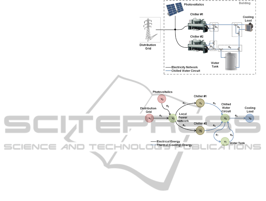
4 ILLUSTRATIVE EXAMPLE
In this section, an example of the definition of a MG
in abstract frameworks described in sections 2 and 3
is introduced. Figure 1 shows small scale MG that
consists of several devices and includes two energy
types - electrical and thermal energy. The MG is
connected to the main distribution grid and includes
the local power source (photovoltalic panels). Two
chillers transform the electricity onto cooling energy
that supplies cooling load or can be store in water
tank. The cooling energy is distributed by water dis-
tribution circuits. Valves divide the cooling energy
from chillers between the water tank and the cooling
load.
Figure 1: Example of a MG.
Figure 2: Graph Representation of the Microgrid.
Microgrid in Graph Representation. Figure 2
shows the graph representation of the considered MG
according to the notation introduced in Section 2.
Distribution grid and photovoltalics are two source
units V
in
=
{
v
1
, v
2
}
that supply the MG with electrical
energy. Local power network v
3
∈ V
m, f
constitutes
the transfer unit that interconnects power generation
and consumption side represented by two chillers
v
4
, v
5
∈ V
m,c
. Chillers are transformation units which
consume electricity and produce cooling (thermal)
energy. Chilled water circuit represented by transfer
unit v
6
∈ V
M, f
transfer cooling energy from chillers
to terminal units v
8
∈ V
out
. Water tank is an energy
storage where thermal energy can be stored and can
be later utilized. Because water tank v
7
∈ V
m
oper-
ates with same type of energy is considered as spe-
cial case of transfer unit V
m, f
. Valves s
1
, s
2
, s
3
, s
4
are part of the setting r affecting energy flows P
f
on the graph’s edges E. The r involves also (i) the
chillers’ commitment o, (ii) chillers’ input power con-
trol l. Control of the storage tank is already cover
by the valves s
4
. Therefore setting r can be writ-
ten as r ≡ (s
1
, s
2
, s
3
, s
4
, o(v
4
), o(v
5
), l). Energy man-
agement systems has to ensure satisfaction of cool-
ing load via modulating of bypassing valves and via
suitable chillers’ and commitment. From the internal
states, we will consider only the state of the storage
tank S(v
7
) = {p} that is considered as cooling en-
ergy of the tank. Let its index be p, then we write
the actual value of the water tank state (stored en-
THEMICRO-GRIDASASTOCHASTICHYBRIDSYSTEM-TwoFormalFrameworksforAdvancedComputing
143

ergy) as P
ch
(t) ≡ H(v
7
, p,t). As the disturbances we
consider the ambient temperature, solar radiation, and
building’s occupancy, i.e. d = (T
oa
, h, o). All of them
can be considered as realization of random processes
over (Ω, F , P ) and foretasted, potentially by exter-
nal providers (weather). Based on these forecasts, ex-
pected cooling loads P
d
(v
8
) and photovoltalics gener-
ation P
s
(v
2
,t) can be estimated and consequently used
for optimization. The grid power supply P
s
(v
1
,t) is
considered as subject of control. In case of tran-
sitions units, i.e. v
3
and v
6
, the outputs depend on
l(t), respectively on the valves s
1
, s
2
, s
3
, s
4
. Finally
the discharging power flow P
f
(e
8
,t) from the water
tank is determined by the state of charging S(v
7
,t)
and the discharging control is given by valve s
4
. The
cost model C is the same as introduced in general in
the previous section. The link functions ξ are in case
chillers are based on the COP curves , depending on
the input power flows (P
f
(e
3
,t) and P
f
(e
4
,t)) and the
ambient temperature d
1
≡ T
oa
. In case of transitions
units, i.e. v
3
and v
6
, the outputs depend on l(t), re-
spectively on the valves s
1
, s
2
, s
3
, s
4
. Finally the dis-
charging power flow P
f
(e
8
,t) is determined by the
state of charging S(v
7
,t) and the discharging control
k(t). The cost model C is the same as introduced in
general in the previous section.
Microgrid as GSHS. In this section, relation be-
tween GSHS defined in Section 3 and given example
of the MG is described. Set of discrete states Q is
given by commitment o, i.e. Q = {0, 1}
2
. Mapping
n : Q → N determines the dimension that remains al-
ways the same, since the continuous state x involves
d, r, (P
f
)
e∈E
, P
ch
, P
d
(v
9
),C in all the cases. The dis-
crete dynamics is represented as decisions about the
commitment o. They determine the sequence of stop-
ping times T that change operation of the MG.
The continuous dynamic can constitute thermal
properties of water, dynamical behavior of chillers
etc. Diffusion term σ constitutes stochastic influences
affecting continuous dynamic b, both are related to
the functions δ, ζ, ρ and ξ. In given example, cooling
load is considered as a stochastic process that can not
be controlled and can be described by (8).
5 POTENTIAL APPLICATIONS
Microgrid modeled as a stochastic hybrid system can
be used for investigation whether given system can
reach undesired discrete modes. Model checking the-
ory offers methods for investigation, not only whether
given model can reach given state, but with what
probability as well (Baier and Katoen, 2008).
Important role of MG energy management system
is to minimize of operational costs of a MG with sat-
isfaction of supplies to all loads. This can be achieved
by suitable scheduling and utilization of internal and
external energy sources. Adopting of a SHS frame-
work for MG modeling, we can use methods related
to SHS theory for solving of a scheduling problem,
e.g. via the scenario approach (Campi et al., 2009).
6 CONCLUSIONS AND FUTURE
WORK
Objective of this paper is not to model particular parts
of a MG, but offers better insight into two formal
abstract framework where a MG can be modeled.
Graph representation is more less traditional point of
view to a MG which is motivated by practical realiza-
tion of MG’s energy management solutions. This rep-
resentation was formalized in Section 2. Stochastic
hybrid systems were introduced in Section 3 and con-
stitutes a framework for multidisciplinary modeling.
Considering MGs as SHS, the definitions and models
would have to be developed in more detail, especially
regarding the continuous dynamics. A high level ex-
ample of modeling a simple MG in both frameworks
was showed in Section 4. Finally, Section 5 sketches
out the benefit of considering MG as a SHS, namely
model checking examining extreme situations in the
system and stochastic dynamic programming for effi-
cient scheduling.
ACKNOWLEDGEMENTS
Research was supported by the European Commis-
sion under the project MoVeS, FP7-ICT-257005.
REFERENCES
Baier, C. and Katoen, J.-P. (2008). Principles of Model
Checking (Representation and Mind Series). The MIT
Press.
Bujorianu, M. and Lygeros, J. (2006). Toward a general
theory of stochastic hybrid systems. Lecture Notes in
Control and Information Sciences (LNCIS), 337:3–30.
Campi, M. C., Garatti, S., and Prandini, M. (2009). The sce-
nario approach for systems and control design. Annual
Reviews in Control, pages 149–157.
Chowdhury, S., Chowdhury, S., and Crossley, P. (2009). Mi-
crogrids and Active Distribution Networks, volume 6
of Renewable Energy Series. The Institution of Engi-
neering and Technology.
SMARTGREENS2012-1stInternationalConferenceonSmartGridsandGreenITSystems
144