
Novel Channel Estimation Algorithm using Various Filter Design in
LTE-Advanced System
Saransh Malik, Sangmi Moon , Bora Kim, Cheolhong Kim and Intae Hwang
Department of Electronics and Computer Engineering, Chonnam National University,
300 Yongbong-Dong, Buk-Gu, Gwangju, Republic of Korea
Keywords: Channel Estimation, OFDM, LTE-Advanced.
Abstract: Channel estimation is a major issue in communication system. In this paper, we propose a new idea for
channel estimation that uses a Kalman Filter (KF) approach to predict the channel in OFDM symbols with
pilot subcarriers where channel affected is by high doppler spread. We design the algorithm considering the
lattice-type arrangement of pilot subcarriers in a LTE-Advanced system from 3GPP. In further advancement,
we use the filtering of channel impulse response and application of a Wiener Filter for the estimation of the
channel frequency response in the rest of the subcarriers.
1 INTRODUCTION
There are several techniques used to estimate the
channel in a wireless communication system. The
effectiveness of these techniques depends on key
factor such as the environment (indoor, outdoor,
rural, urban) and the mobility between transmitter
and receiver. Primarily, least square (LS) estimation
is the most simple of the conventional channel
estimations techniques, but it only works well for
time-invariant channels or with low Doppler spread.
Minimum mean squared error (MMSE) combined
with a linear interpolation method is more effective
than LS because it considers the channel correlation
values. However for time-variant channels, it is
necessary to implement techniques able to estimate
or predict the variations of the channel in time, such
as Wiener and Kalman filters. In this research, we
want to proposed a method to estimate and predict
the variations of channel in fast fading channels,
considering the especial arrangement of reference
signals in LTE, since other papers are usually based
on block-type or comb-type arrangements.
This paper is divided as follows, section II shows
the arrangement of reference signals in 3GPP-LTE
advanced, section III briefly describes conventional
channel estimation methods, section IV describes
our proposal, section V shows our simulation results
and finally section VI contains our conclusions.
2 REFERENCE SIGNAL IN LTE-
ADVANCED
LTE-Advanced uses signals known by both the
transmitted and the receiver, sent in predefined
locations. This signals are called downlink reference
signals (3 GPP TS 36.211, 2010). By processing the
received reference signals, the receiver can estimate
the whole channel response for each OFDM symbol.
In the time-domain, for one antenna port,
reference signals are transmitted during the first and
fifth OFDM symbols of each slot when the normal
cyclic prefix (CP) is used and during the first and
fourth OFDM symbols when the extended CP is
used. In the frequency-domain, they are inserted
every six subcarriers.
2.1 Relationship between Coherence
Bandwidth and Reference Signals
In 3GPP LTE
Table 1: Delay profile for 3GPP LTE channel model.
Channel
Number of
Chanel Taps
Delay Spread
(r.m.s)
Max. Excess
Tap delay
EPA 7 45ns 410 ns
EVA 9 357ns 2510 ns
ETU 9 991ns 5000 ns
120
Malik S., Moon S., Kim B., Kim C. and Hwang I..
Novel Channel Estimation Algorithm using Various Filter Design in LTE-Advanced System.
DOI: 10.5220/0004026901200125
In Proceedings of the International Conference on Signal Processing and Multimedia Applications and Wireless Information Networks and Systems
(SIGMAP-2012), pages 120-125
ISBN: 978-989-8565-25-9
Copyright
c
2012 SCITEPRESS (Science and Technology Publications, Lda.)

Figure 1: Mapping of Downlink reference signals for one
antenna port in extended CP.
Table 2: Coherence bandwidth of 20 MHz LTE-Advanced
system.
Channel B
(0.9)
B
(0.5)
EPA 1.6 MHz 3.7 kHz
EVA 201.1 kHz 466.9 kHz
ETU 72.4 kHz 168.2 kHz
In LTE-Advanced, the subcarrier space frequency Δf
is 15 kHz. Since the reference signals in the
frequency domain are located every 6 subcarriers,
the reference signal bandwidth is 90 kHz. If the
channel frequency response remains constant, the
correlation in the frequency domain should have a
value close to 1; while we choose a value of 0.5 as
an indicator that the channel has changed. Based on
this assumptions, we can estimate the coherence
bandwidth for both situations using equation (1)
(Somasegeran, 2007):
)arccos(
2
1
c
s
πτ
β
≥
(1)
where c is the correlation in frequency domain, and
τ
s
is the root-mean-square (RMS) delay spread given
for LTE extended channel models: Extended
Pedestrian A (EPA), Extended Vehicular A (EVA)
and extended urban (ETU) channels (Table 1).
The results in Table 2 demonstrate that, basically,
the channel is constant during the bandwidth
corresponding to the spacing of reference symbols in
frequency domain; and therefore, the reference
signals in LTE-Advanced are able to keep track of
the frequency selective fading.
2.2 Relationship between Coherence
Time and Reference Signals in
3GPP LTE
For the extended cyclic prefix case, there are 6
symbols in 1 slot (12 symbols per sub frame).
Therefore, we can calculate 1 OFDM symbol period
as:
s
ms
N
T
T
symb
slot
symb
μ
3.83
6
5.0
===
Reference signals are transmitted during the first and
fourth OFDM symbols in each slot. Therefore, the
spacing of reference signals in time domain is:
msTT
symbref
25.0.3 ==
Table 3: Maximum doppler frequency for 3 GPP LTE–
Advanced channel models.
Channel
Maximum Doppler
Frequency (Hz)
UE Maximum Speed (Km/h)
*carrier frequency 2 GHz
EPA 5 3
EVA 70 40
ETU 300 160
If the channel is constant in time, the correlation
in the time domain should be close to 1; as such we
choose a value of 0.5 as an indicator that the channel
has changed. Based on these assumptions, we can
estimate the coherence time for both situations,
using equation (2) and the maximum Doppler
frequency corresponding to the LTE-Advanced
channel models as shown in Table 3.
)arccos(
2
1
c
f
t
D
c
π
=Δ
The results shown in Table 4 demonstrate that the
spacing of reference symbols in time is less than the
coherence time; therefore, the reference signals in
LTE are able to keep track of the time-varying
fading channel.
Table 4: Coherence time 20 MHz 3GPP LTE-Advanced
system.
Maximum Doppler Frequency Δt
(0.9)
Δt
(0.5)
f
D
= 5 Hz 14.4 ms 33.3 ms
f
D
= 70 Hz 1.0 ms 2.4 ms
f
D
= 300 Hz 0.2 ms 0.6 ms
The results shown in Table 4 demonstrate that
the spacing of reference symbols in time is less than
the coherence time; therefore, the reference signals
in LTE are able to keep track of a time-varying
fading channel.
NovelChannelEstimationAlgorithmusingVariousFilterDesigninLTE-AdvancedSystem
121

3 CONVENTIONAL CHANNEL
ESTIMATION METHODS
In this section we briefly describe conventional techniques
to estimate and/or predict the channel frequency response
(CFR)
.
3.1 LS Channel Estimation
LS is the simplest method to estimate the channel.
First, we calculate the CFR only in the subcarriers
that contain reference symbols. We do so, by
dividing the received reference signals between their
transmitted value (Simko, 2009):
()
()
(
)
()
()
()
⎥
⎥
⎦
⎤
⎢
⎢
⎣
⎡
=
∧
pp
pp
p
p
p
p
LSp
Nx
Ny
x
y
x
y
H ...
2
2
,
1
1
,
(3)
The channel frequency response for the rest of the
subcarriers, is estimated with interpolation and
extrapolation in frequency and time dimensions.
Figure 2: Block Diagram of LS Channel Estimation
3.2 MMSE Channel Estimation
Another method to estimate the channel is the
MMSE algorithm which has better performance than
LS but is computationally
more complex. MMSE
calculates the channel impulse response that
minimizes the mean square error between the actual
and estimated channel impulse response (Hou and
Liu).
The channel in the frequency domain can be
estimated with equation (4):
[]
LSp
H
pphp
MMSEp
HXXRRH
,
1
12
,
)(
∧
−
−
∧
+=
σ
(4)
where is the noise variance, is the cross-
correlation matrix between all subcarriers and the
subcarriers with reference signals within the same
OFDM symbol,
is the autocorrelation matrix of
the subcarriers with reference signals within the
same OFDM symbol, and the superscript
denotes Hermitian transpose. By replacing
in (4) with its expectation , the
MMSE channel estimator in frequency domain can
be expressed as:
LSp
ppphp
MMSEp
HI
SNR
RRH
,
1
,
∧
−
∧
⎥
⎦
⎤
⎢
⎣
⎡
+=
β
(5)
where is a constant depending on the type of
modulation and β is the identity matrix. We can
estimate the channel for the other resource elements
using linear interpolation in time domain.
Figure 3: Block diagram of MMSE channel estimation.
3.3 Wiener Filter
The Wiener Filter (WF) uses the same principle than
MMSE method (Qin et al., 2007) and it also
eliminates noise effects in the channel estimation.
WF allows us to keep track of the variations of the
CIR in time-variant channels because it uses both
the time and frequency correlations.
To simplify the complexity, the 2-dimensional
WF is decompose into two separated WF's; one in
the frequency domain and one in the time domain.
First, we obtain directly the channel estimation in
frequency domain for the OFDM symbols with
reference signal as:
LSp
p
f
pp
f
hp
f
MMSEp
HI
SNR
RRH
,
1
,
∧
−
∧
⎥
⎦
⎤
⎢
⎣
⎡
+=
β
(6)
Then we estimate the total channel frequency for all
OFDM symbols using WF in time domain:
f
WF
p
t
pp
t
pp
WF
HI
SNR
RRH
∧
−
∧
⎥
⎦
⎤
⎢
⎣
⎡
+=
1
β
(7)
Figure 4: Block diagram 2x1 dimensional WF.
3.4 Kalman Filter
The purpose of the Kalman Filter (KF) is to use
measurements observed over time, containing noise,
and produce values that are closer to the true values
of the measurements and their associated calculated
SIGMAP2012-InternationalConferenceonSignalProcessingandMultimediaApplications
122
values. In this section, we study the KF that is used
to predict variations of the channel in time domain
and which can also be applicable to frequency
domain.
The principle behind KF applied to channel
estimation is that we can represent the channel
frequency response, at time, as an infinite order
autoregressive (AR) process (Karakaya et al., 2009).
Figure 5: System using KF and block type pilot
arrangement.
Where, k and A are the order and the coefficient
of the AR process, respectively. V is a white
Gaussian noise with zero mean and variance σ
2
. For
the case of first order AR process
and .
In order to reduce the computational complexity,
only the first order AR process, i.e., is considered.
Therefore, we can represent the vector form of the
channel frequency response at time n as:
Then, the channel estimate can be obtained by a
set of recursions (Ling and Ting, 2006):
The received symbol at time can be expressed in the
form of a linear regression model.
4 PROPOSED CHANNEL
ESTIMATION SCHEME
In this section introduce and explain the proposed
method to predict the channel in high Doppler
spread.
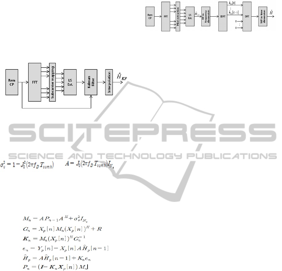
Fig. 6 shows the New Channel Estimator's block
diagram that was designed considering the lattice-
type reference signals arrangement of 3GPP LTE (so
far most of the studies focus on block-type or comb
type pilot arrangements).
Figure 6: Block diagram of the new channel estimator.
After FFT, the reference signals or pilots of the
first OFDM symbols are extracted and we can
estimate the channel frequency response (CFR)
using a simple method, such as LS. Using the
recursions of KF, we can estimate the variation of
CFR for the later OFDM symbols containing
reference signals. Then, we transform the CFR into
CIR and eliminate the taps with index larger than L;
this way we eliminate the noise contained in those
taps. Finally, we transform the CIR to CFR and
estimate the channel for the rest of the subcarriers
using WF in time dimension.
5 SIMULATION RESULTS
In this section we show the performance analysis of
channel estimation methods. The simulations are
performed in MATLAB using the simulation
parameters of 3GPP LTE-Advanced shown in Table
5. The time variant channel is modelled according to
the values given for LTE extended channel models
in Table 1 and the maximum Doppler Frequency
values for each channel given in Table 3. The
frequency power spectrum follows the Jakes model.
Following the results of section II, we assume the
channel to be constant for 1 OFDM symbol.
Fig. 7 shows the BER performance of different
channel estimation methods in EPA channel with
max. Doppler Frequency of 5Hz. For this case, the
motion speed is low; therefore, as shown in sections
II, the channel suffers little variation in time within
one subframe and techniques like LS or MMSE with
linear interpolation produce good results.
Fig. 8 shows the BER performance of different
channel estimation methods in EVA channel with
max. Doppler frequency of 70Hz. In this case, the
mobile user moves with medium speed; therefore, as
shown in section II, the channel suffers more
variation in time within one subframe compared to
the case of EPA. We can observe that the BER
obtained with LS and MMSE starts to separate from
the actual value, but WF and New CE produce more
accurate results.
Fig. 9 shows the BER performance of different
channel estimation methods in ETU channel with
max. Doppler frequency of 300Hz. In this case, the
NovelChannelEstimationAlgorithmusingVariousFilterDesigninLTE-AdvancedSystem
123

mobile user moves with very high speed; therefore,
as shown in section II, the channel suffers significant
variations in time, even within one subframe. We
can observe that the effectiveness of LS and MMSE
is affected by the high Doppler spread; therefore it is
necessary to employ techniques that consider the
time correlation of the channel. We demonstrate
through this simulation that our proposed technique,
New CE, produces the best results for high Doppler
spread environments.
Table 5: Simulation parameters.
Parameter Value
Bandwidth 20 MHz
Sample frequency 30.72 MHz
Subframe duration 1 ms
Subcarrier spacing 15 kHz
FFT size 2048
Occupied subcarriers
1200 + DC subcarrier =
1201
No. subcarriers/RB 12
No. of RB’s/subframe 100
CP size (samples) 512 (extended CP)
No. of OFDM symbols/subframe 12 (extended CP)
No. of reference signals per RB 8
Modulation scheme QPSK
Noise AWGN
No. of antennas 1x1
Channel estimation Techniques
LS with linear interpolation,
MMSE, Wiener Filter,
Creative CE
Channel models
3GPP LTE extended channel
models: EPA, EVA, ETU
Figure 7: BER Performance using different channel
estimation methods in EPA channel with maximum
Doppler frequency of 5 Hz.
Figure 8: BER performance using different channel
estimation methods in EVA channel with maximum
Doppler frequency of 70Hz
Figure 9: BER performance using different channel
estimation methods in Rayleigh ETU channel; with
maximum Doppler frequency of 300 Hz.
6 CONCLUSIONS
In this paper we proposed a novel channel
estimation method to improve transmission and
reception of data in high speed environments. We
designed our system considered the especial
arrangement of reference signals in 3GPP LTE-
Advanced and demonstrated through MATLAB
simulations that the BER performance result in high
Doppler spread is very close to the case of ideal
channel estimation.
SIGMAP2012-InternationalConferenceonSignalProcessingandMultimediaApplications
124

ACKNOWLEDGEMENTS
This research was supported by the MKE(The
Ministry of Knowledge Economy), Korea, under the
ITRC (Information Technology Research Center)
support program supervised by the NIPA(National
IT Industry Promotion Agency)" (NIPA-2012-
H0301-12-3005).This study was financially
supported by Chonnam National University, 2011.
REFERENCES
3GPP TS 36.211: "E-UTRA; Physical Channels and
Modulations", v 9.1.0, March 2010.
L. Somasegaran, "Channel Estimation and Prediction in
UMTS LTE", Master Thesis, Aalborg University,
Denamrk, Feb. 22nd - June 25th 2007, 2
nd
edition.
M. Simko, "Channel Estimation for UMTS Term Long
Evolution", Master Thesis, Vienna University of
Technology, Austria, June 2009.
J. Hou, J. Liu, "A Novel Channel Estimation Algorithm
for 3GPP LTE Downlink System Using Joint Time-
Frequency Two-Dimensional Iterative Wiener Filter",
University of Science and Technology of China.
Y. Qin, B. Hui, K. Chang, "Novel Pilot-Assisted Channel
Estimation Techniques for 3GPP LTE Downlink with
Performance-Complexity Evaluation", Korean
Conference on Digital Communications, vol. 37, no. 7,
Oct. 2007.
B. Karakaya, H. Arslan, H. Cirpan, "An Adaptive Channel
Interpolator Based on Kalman Filter for LTE Uplink
in High Doppler Spread Environments.", EURASIP
Journal on WIreless Communications and
Networking, vol. 2009, article ID 893751.
W. Ling, L. Ting, "Kalman filter channel estimation based
on comb-type pilot in time-varying channel",
International Conference on Wireless
Communications, Networking and Mobile Computing
(WiCOM), Sept. 2006.
NovelChannelEstimationAlgorithmusingVariousFilterDesigninLTE-AdvancedSystem
125
