State Dependent Parameter Modelling of a DC-DC Boost Converter in
Discontinuous Conduction Mode
U. Hitzemann
1
and K. J. Burnham
1,2
1
Control Theory and Applications Centre, Coventry University, Coventry, U.K.
2
Faculty of Electronics, Wroclaw University of Technology, Wroclaw, Poland
Keywords:
DC-DC Boost Converter, Nonlinear Circuits, State-dependent Parameter Modelling, System Identification,
System Modelling.
Abstract:
This paper is concerned with the modelling of a DC-DC boost converter, operating in discontinuous conduction
mode (DCM). The approach chosen is to model the converter using a state-dependent parameter (SDP) model
approach which is expected to be able to deal with the nonlinearities of the system, as well as a varying load.
The modelling procedure presented, makes use of input-output data only and no physical insight into the
system is required. Results are verified via laboratory experiments.
1 INTRODUCTION
DC-DC boost converters are switched mode power
electronic devices. The boost converter steps up a DC
input voltage to a higher DC output voltage. Hence
they find their application where a higher, controlled
DC voltage than the supply voltage is required; this
being the case, e.g. in DC-motor drive applications or
power distribution systems.
The difficulty in modelling a DC-DC converter
lies in its hybrid nature due to the switching pro-
cess. There are two conditions which are required to
be considered, namely, when the switch is open and
when the switch is closed. In discontinuous conduc-
tion mode (DCM), an additional condition of the con-
verter is required to be taken into account, i.e. when
the switch is open and the inductor is not conducting.
In the literature, the common approach used to
model a DC-DC converter is the state-space averag-
ing method (Middlebrook and Cuk, 1976; Erickson
and Maksimovic, 2001; Sun et al., 2001; Xie et al.,
2010), where each of the conditionsare modelled sep-
arately and the models are averaged over the entire
period. The models are usually obtained by making
use of physical relationships. Often, however, an ex-
act physical insight into the converter is not necessar-
ily available, due to the tolerances of the components
and their inherent parasitic elements. The approach
considered in this paper requires no physical insight
since the modelling process makes use of the input -
output data only. Additionally, the ‘linear-like’ struc-
ture of the state-dependent parameter (SDP) model
(see (Young, 2000)) makes it suitable in the design
of model based controllers, allowing linear control
theory to be used. This is not necessarily the case
when making use of models based on physical rela-
tionships. In several practical systems, model based
control, such as the proportional integral plus con-
troller (PIP), based on SDP models has already been
successfully applied (Taylor et al., 2007). All results
presented here are verified via experiments using a
practical, laboratory based DC-DC boost converter.
The paper is organised as follows: A brief descrip-
tion of the boost converter is given in Section 2. The
SDP model of the converter is obtained in Section 3.
Conclusions are given in Section 4.
2 DC-DC BOOST CONVERTER
In this Section, the boost converter is briefly intro-
duced. Figure 1 shows the topology of a boost con-
verter with ideal components, where L, C, S and R
denote the inductor, the capacitor, the switch and the
load represented by a resistor, respectively. The quan-
tities V
i
, V
o
, v
L
and v
C
denote the input voltage, the
output voltage, the voltage across the inductor and
the voltage across the capacitor, respectively. The
switch, represented by a MOSFET, is driven by a
pulse-width-modulated (PWM) voltage with a duty-
482
Hitzemann U. and J. Burnham K..
State Dependent Parameter Modelling of a DC-DC Boost Converter in Discontinuous Conduction Mode.
DOI: 10.5220/0004034704820487
In Proceedings of the 9th International Conference on Informatics in Control, Automation and Robotics (ICINCO-2012), pages 482-487
ISBN: 978-989-8565-21-1
Copyright
c
 2012 SCITEPRESS (Science and Technology Publications, Lda.)

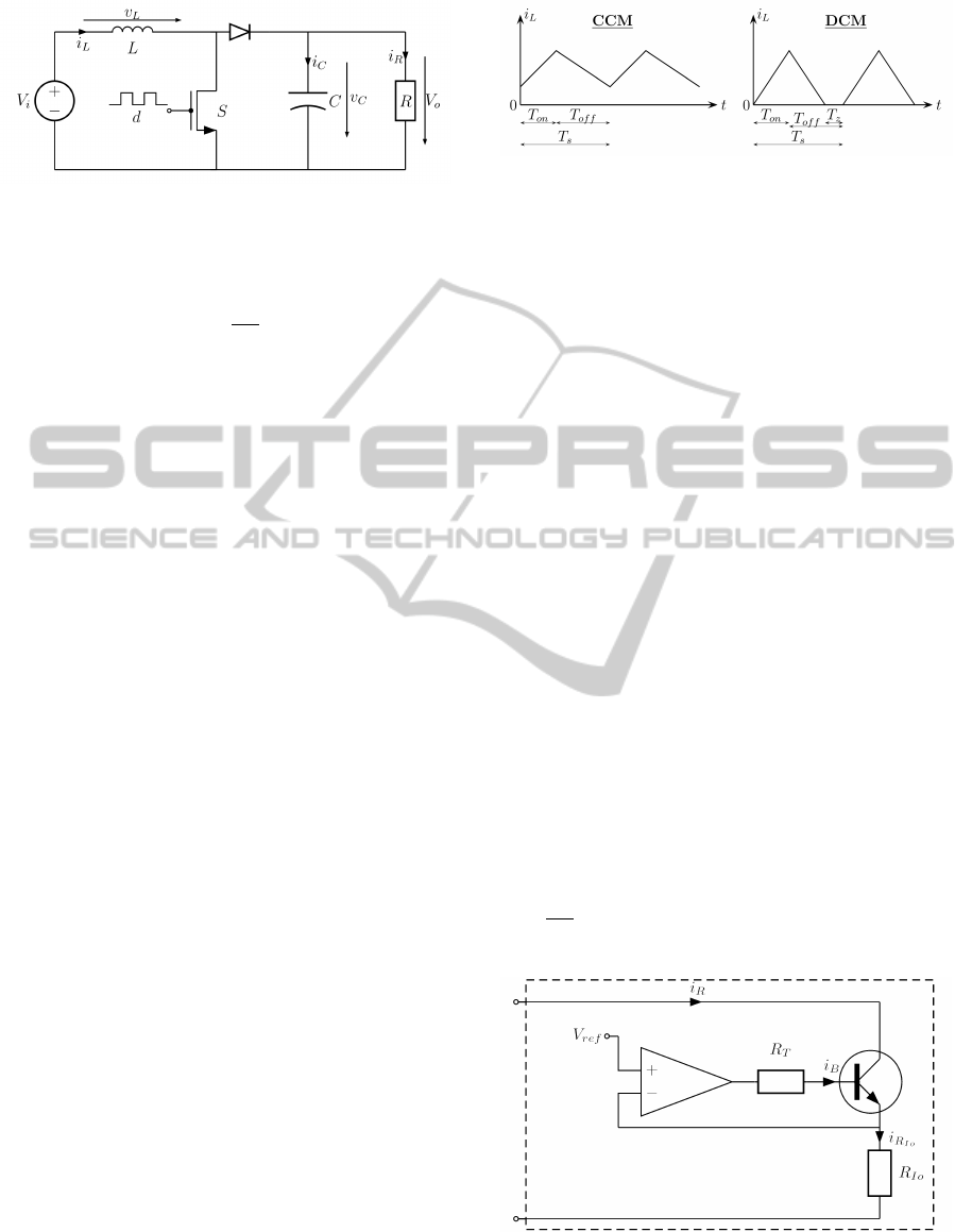
Figure 1: Topology of a DC-DC boost converter with ideal
components.
cycle, denoted d, which is defined as
d =
T
on
T
s
(1)
where T
s
= T
on
+ T
of f
denotes the period of the PWM
signal. The time interval, denoted T
on
, when the
PWM signal is high, corresponds to the switch con-
ducting, while T
of f
corresponds to the time interval
when the PWM signal is low and to the switch not
conducting.
Additionally, the duty-cycle of a PWM signal can
only vary between 0% and 100% so that d is defined
to be in the per-unit range
{d ∈ R | 0 < d ≤ 1} (2)
In the following, a brief description of the principle
of operation is provided. The inductor and the capac-
itor are energy storage components. When the switch
is closed, during T
on
, the inductor is charged and only
the capacitorsupplies the load while the diode ensures
that no current is able to flow from the capacitor via
the switch to ground, i.e. a short circuit across the
capacitor. When the switch is open, during T
of f
, the
energy stored in the inductor is transferred to the ca-
pacitor and to the load. Consequently, when consid-
ering the law of energy conservation, it can be con-
cluded that the output voltage V
o
can be influenced by
the duty-cycle of the PWM signal. For detailed infor-
mation, see e.g. (Erickson and Maksimovic, 2001).
2.1 Operational Modes
In general, the converter either operates in continuous
conduction mode (CCM) or in DCM. However, the
latter is considered in this paper only. The difference
is that in CCM, the inductor current is always greater
than zero, as shown in Figure 2, where the inductor
continuously conducts current. In DCM, the inductor
current settles to zero and remains at this value until
the end of the period. This time interval is denoted by
T
z
.
Figure 2: Idealised inductor current in CCM and in DCM.
2.2 Converter Set-up
The set-up of the prototype converter used for lab-
oratory experiments is as follows: V
i
= 5V, L =
745µH with inherent series resistance of ≈ 1.3Ω and
C = 1mF. For DCM operation, the switching pe-
riod, which is also equivalent to the sampling inter-
val, is chosen to be T
s
= 1ms. In order to generate
the PWM signal and to obtain the required measure-
ments, the dSPACE MicroAutobox DS1401 is used.
The maximal measurable output voltage V
o
is limited
to V
o
= 20V, hence the output voltage is defined to be
in the range
{V
o
∈ R | 5V ≤ V
o
≤ 20V} (3)
The maximum current, which can be delivered by the
power supply is limited, hence the value i
L
= 2A can-
not be exceeded.
The load, represented by R in Figure 1, is realised
as shown in Figure 3. This allows the output currenti
R
to be determined by applying a load reference voltage
V
ref
. This is provided by the DS1401 digital to ana-
log converter. The resistor R
Io
= 10Ω is assumed to
be accurately known. The operational amplifier regu-
lates the resistance of the transistor via R
T
= 220Ω in
such a way, that the voltage across the resistor R
Io
is equal to V
ref
and the output current is given by
i
R
=
V
ref
R
Io
provided that the base current i
B
<< i
R
, so
that i
R
= i
R
Io
.
Figure 3: Realisation of the load R (dashed box).
Realising the load in this way, provides the oppor-
tunity of considering different loading scenarios.
StateDependentParameterModellingofaDC-DCBoostConverterinDiscontinuousConductionMode
483

Due to the above mentioned hardware limitations,
and in order to ensure DCM operation, the output cur-
rent is defined to be in the range
{i
R
∈ R | 40mA ≤ i
R
≤ 140mA} (4)
3 SDP – MODEL
The converter is referred to in the following as the
system, and the modelling approach is based on mea-
sured input-output data. These are obtained by ap-
plying a staircase input signal to the system of an ap-
propriate step height. Furthermore, the output cur-
rent is kept constant during each staircase response.
Then, the output current is incremented and the pro-
cedure is repeated. The value of the output current
starts at i
R
= 40mA and is incrementally increased
to 140mA in steps of 10mA. The input step height
in each staircase response is required to be chosen ap-
propriatelyin order to obtain sufficient step responses,
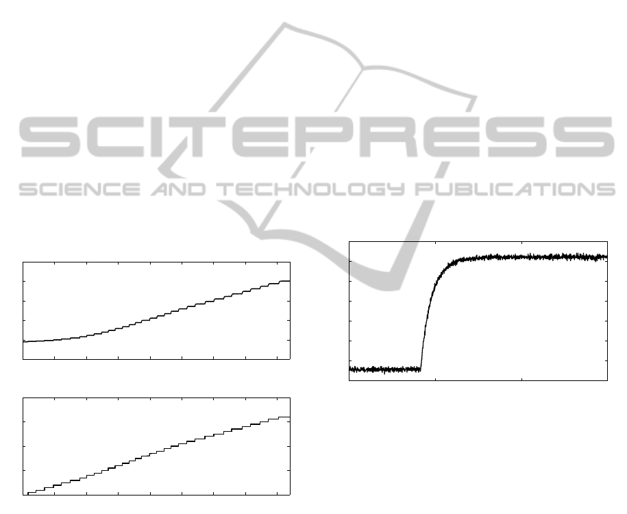
covering the entire operating range. An exemplary
yet representative staircase input and corresponding
measured output voltage are shown in Figure 4, when
i
R
= 100mA. Based on these input-output data, the
modelling procedure is performed.
0 1 2 3 4 5 6 7 8
x 10
4
0
5
10
15
20
25
0 1 2 3 4 5 6 7 8
x 10
4
0
0.2
0.4
0.6
0.8
Output Voltage [V]
Duty-Cycle
Samples
Figure 4: Measured output voltage response (upper) to the
staircase input signal (lower) with constant output current
value of i
R
= 100mA.
3.1 SDP structure
Consider the following system equation
y
k
+ a
1
(s
k
)y
k−1
+ . . . + a
n
a
(s
k
)y
k−n
a
= b
1
(s
k
)u
k−1
+ . . . + b
n
b
(s
k
)u
k−n
b
(5)
where y
k
and u
k
denote the system output voltage
and system input, i.e. the duty-cycle, respectively.
s
k
indicates, that the parameters are functions of one
or more elements of the non- minimal state vector
(Young et al., 1987; Wang and Young, 1988), i.e. sys-
tem output voltage and system input, and/or functions
of other variables, see (Young, 2000).
In addition, by adopting the SDP model struc-
ture (5), the ‘frozen’ linear system, as defined by
the SDP model at every sampling instant, can form
the basis for state dependent control system design
based on linear control methods (Kontoroupis et al.,
2003). However, global stability cannot be guaran-
teed if there is model mis-fit (Taylor et al., 2009) and
so the closed loop system must be investigated care-
fully in this regard.
3.2 System Identification
From the staircase responses, as shown in Figure 4,
and, in particular, the individual steps of the staircase,
as shown in Figure 5, it can be concluded that a first
order system model is an adequate choice, i.e. n
a
=
n
b
= 1. This means, that only the parameters a
1
(s
k
)
and b
1
(s
k
) are required to be identified.
3.95 4 4.05 4.1
x 10
4
9.9
10
10.1
10.2
10.3
10.4
10.5
10.6
Output Voltage [V]
Samples
Figure 5: Magnified single step of the staircase response
shown in Figure 4.
Initially, the steady-state behaviours for each out-
put current are modelled. The function, which de-
scribes the steady-state behaviours is found empiri-
cally to be of the polynomial form
y
j,∞
(u
∞
) =
4
∑
l=1
β
j,l
u
4−l
∞
(6)
where j = 1, 2, . . . , 10, which corresponds to the out-
put currents i
R
= 40mA, 50mA, . . . , 140mA. y
j,∞
and
u
∞
denote the steady-state output and input, respec-
tively. The parameters β
j,l
are identified by making
use of the least-squares algorithm, see e.g. (Hsia,
1977). At this point, it is noted that the parameters
β
j,l
can be formulated as functions of the output cur-
rent. Again, the function is found empirically to be of
ICINCO2012-9thInternationalConferenceonInformaticsinControl,AutomationandRobotics
484

the polynomial form
β
l
(i
R
) =
4
∑
f=1
γ
l, f
i
4− f
R
l = 1, 2, . . . , 4 (7)
where i
R
is in mA. The constant parameters γ
l, f
are
identified, by making use of the least-squares method.
Substituting (7) into (6) yields the modelled steady-
state behaviour of the system that is dependent on the
output current
y
∞
(i
R
, u
∞
) =
4
∑
l=1
β
l
(i
R
) u
4−l
∞
(8)
The steady-state output against the steady-state input
is shown in Figure 6, where each trace, from left to
right, correspondsto the output currents of fixed value
i
R
= 40mA, 50mA, . . . , 140mA. The steady-state be-
haviour obtained from measurements are compared
against the identified polynomials (6) (solid lines)
and against the polynomial where the coefficients are
modelled as output current dependent quantities (8)
(dashed line). It can be observed, that the mismatch at
high output currents and high voltages increases. Fig-
ure 7 shows the parameters obtained from (6) (solid
line) and the estimated, output current dependent pa-
rameters according to (7) (dashed line).
Having characterised the steady-state behaviour,
the next step is to consider the transients, and the
system parameter a
1
(s
k
) is required to be identified.
Since this parameter is not measurable directly, each
step of each staircase response is considered individ-
ually. Here, a first order linear model of the form (5),
but with invariant parameters, is identified by making
use of the least-squares algorithm. In this way, a
1
(s
k
)
at several points through the entire operating range
is obtained. The estimated system parameter values
0 0.1 0.2 0.3 0.4 0.5 0.6 0.7 0.8 0.9
4
6
8
10
12
14
16
18
20
22
40 mA, 50 mA, ⋅⋅⋅ , → 140 mA
measured
fitted Polyn.
estimated
Steady-State Output [V]
Steady-State Input
Figure 6: Steady-state behaviour, measured and modelled
by fitting polynomials (solid lines) as well as modelled by
a polynomial incorporating the output current (dashed line),
for output currents starting at i
R
= 40mA increasing in steps
of 10mA up to i
R
= 140mA, from left to right.
40 50 60 70 80 90 100 110 120 130 140
−400
−200
0
40 50 60 70 80 90 100 110 120 130 140
0
200
400
40 50 60 70 80 90 100 110 120 130 140
2
3
4
40 50 60 70 80 90 100 110 120 130 140
4
4.5
5
Output current [mA]
β
1
β
2
β
3
β
4
Figure 7: Parameters of (8) β
l
obtained as a function of the
output current (7) (dashed line) and obtained directly from
considering the individual steady-state behaviours (6) (solid
line).
a
1
(s
k
) are shown in Figure 8, where each trace cor-
responds to the staircase responses obtained for each
output current value i
R
= 40mA, 50mA, . . . , 140mA.
The output current dependency of the system param-
eter a
1
(s
k
), which is also a measure of the time con-
stant of the system, is not immediately obvious in the
discrete time domain, as shown in Figure 8. The dif-
ferences of the traces seem to be marginal, in par-
ticular with increasing output voltage. This means
that since each trace corresponds to a certain con-
stant output current, the output current dependency
on the system parameter a
1
(s
k
) would apparently ap-
pear to be insignificant. For this reason, an aver-
aged function, independent of the output current, de-
scribing a
1
(s
k
) was used in (Hitzemann and Burn-
ham, 2011). This implies, that the transient behaviour
of the converter does not depend on the output cur-
rent significantly. However, to highlight the depen-
dency, Figure 9 shows the time constant τ of the sys-
tem against the output voltage, where, again, each
trace corresponds to a certain value of the output cur-
4 6 8 10 12 14 16 18 20
−1
−0.95
−0.9
−0.85
−0.8
−0.75
System parameter a
1
(s
k
)
Output Voltage [V]
Figure 8: System parameter a
1
(s
k
) against the output volt-
age where each trace corresponds to the output current val-
ues i
R
= 40mA, 50mA, . . . , 140mA.
StateDependentParameterModellingofaDC-DCBoostConverterinDiscontinuousConductionMode
485

4 6 8 10 12 14 16 18 20
0
0.05
0.1
0.15
0.2
0.25
0.3
0.35
Time Constant τ [s]
Output Voltage [V]
Figure 9: Time constants, obtained from staircase responses
directly (solid line) and estimated (dashed line), against the
output voltage. Each trace corresponds to a fixed output cur-
rent i
R
= 40mA, 50mA, . . . , 140mA, from upper to lower.
rent i
R
= 40mA,50mA, . . . , 140mA. Here, the output
current dependency of the time constant and hence of
a
1
(s
k
) is clearly discernable. Additionally, it can be
observed, that the spread of the traces increases when
the output voltage increases. Hence, it can be deduced
that the output current dependencyof the transient be-
haviour does in fact increase when the output voltage
increases.
Due to the approximately linear nature of the time
constant with respect to the output voltage, consider-
ing a constant output current, the following function
is obtained.
τ
j
= α
j,1
y
∞
+ α
j,2
j = 1, 2, . . . , 10 (9)
In order to incorporate the output current dependency,
the parameters α
j,1
= α
1
(i
R
) and α
j,2
= α
2
(i
R
) are as-
sumed to be functions of the output current, cf. in
a similar manner to modelling the steady-state be-
haviour described above
α
f
(i
R
) =
4
∑
l=1
η
f,l
i
4−l
R
f = 1, 2 (10)
where η
f,l
∈ R are constant coefficients identified by
the least-squares method. Subsequently, the system
parameter a
1
(s
k
) can be obtained by substituting (10)
into (9), denoted τ(y
k−1
, i
R
), and mapping back to the
discrete time domain via
a
1
(s
k
) = −e
−
T
s
τ(y
k−1
, i
R
)
(11)
The remaining system parameter b
1
(s
k
) is required
to be obtained in order to satisfy the steady-state be-
haviour. Consequently, this parameter is given by
b
1
(s
k
) =
y
k−1
(1+ a
1
(s
k
))
y
−1
∞
(i
R,k
, y
k−1
)
(12)
where y
−1
∞
(i
R,k
, y
k−1
) denotes the inverse function of
(8).
Remark 1. In (12), to avoid division by zero, the sys-
tem output is required to be greater than that value
which causes y
−1
∞
(i
R,k
, y
k−1
) to be zero, hence, the
lower bound of (3) is required not to be exceeded dur-
ing operation. This in turn, prevents the system input
from becoming zero, which is reflected in (2).
Remark 2. In this paper, the functions used in order
to describe the steady-state behaviour, (6) - (8), as
well as the functions used in order to describe the dy-
namic behaviour, (9) and (10), are chosen to be poly-
nomials of third and first order, respectively. Hence,
the identification of the associated constant parame-
ters is straightforward by making use of least-squares
rather than requiring numerical optimisation meth-
ods as used in (Hitzemann and Burnham, 2011).
Remark 3. The presented system identification pro-
cedure linearises the system at several operating
points through the entire operating range and ‘inter-
polation’ is invoked in between. Considering this, the
incremental step height of the output current and the
input steps of the staircase signal are required to be
chosen with care in order to obtain sufficient accuracy
of the resulting overall system model.
3.3 Model Validation
Having obtained a model of the system, an arbitrary
input sequence is applied to both the system and the
model, for validation purposes. An arbitrary output
current is drawn from the system and applied to the
model, which represents a varying load. Figure 10
shows the response of the model and the measured re-
sponse of the system. It can be seen that the model is
capable of replicating the system response adequately.
Nevertheless, steady-state offset errors are observed,
e.g. the peak between ≈ 85s and 90s. Note that when
taking the output current and the output voltage into
account, which are both high, this observation is in
agreement with the results shown in Figure 6.
4 CONCLUSIONS
In this paper, an approach to modelling a DC-DC
boost converter in discontinuous operation mode has
been presented. The state dependent parameter model
structure has been selected. The presented modelling
approach relies on measured input-output data only
and not on the knowledge of physical relationships.
However, this modelling approach requires a constant
output current, independent of the output voltage, to
ICINCO2012-9thInternationalConferenceonInformaticsinControl,AutomationandRobotics
486

0 10 20 30 40 50 60 70 80 90 100
5
10
15
20
0 10 20 30 40 50 60 70 80 90 100
0
100
200
0 10 20 30 40 50 60 70 80 90 100
0
0.5
1
Output Voltage [V]
Output
Current [mA]
Duty-Cycle
Time [s]
Figure 10: Upper: measured output response of the system (solid line) and output response of the model (dashed line) to
arbitrary varying sequences of the input signal and output current. Middle: arbitrary varying output current sequence (solid
line) in the defined range 40mA ≤ i
R
≤ 140mA (dashed lines). Lower: arbitrary varying input sequence.
be drawn from the converter, which is realised by a
load as shown in Figure 3. Furthermore, the asso-
ciated identification steps make use of polynomials,
so that parameters can be identified straightforwardly
by making use of standard system identification algo-
rithms such as least-squares. Additionally, the tran-
sients are modelled by considering the time constants
in the continuous time domain of the equivalent lin-
ear models at several operating points, which are then
mapped back in the discrete time domain. In this
way, the identification of the transient behaviour is
also modelled in a straightforwardway by making use
of linear relationships. The resulting state dependent
parameter model is able to deal with varying loads by
taking the output current into account. Finally, the
state dependent parameter model has been validated
via a laboratory based experiment confirming its ac-
curacy and appropriateness.
REFERENCES
Erickson, R. W. and Maksimovic, M. (2001). Fundamen-
tals of Power Electronics. Kluwer Academics/Plenum
Publishers, New York, 2nd edition.
Hitzemann, U. and Burnham, K. J. (2011). State depen-
dent parameter modelling and control of a dc-dc boost
converter in discontinuous conduction mode. In Pro-
ceedings of the 9th European Workshop on Advanced
Control and Diagnosis, ACD 2011, Budapest, Hun-
gary.
Hsia, T. C. (1977). System Identification: Least-Squares
Methods. Lexington Books, Massachusetts.
Kontoroupis, P., Young, P. C., Chotai, A., and Taylor, C. J.
(2003). State dependent parameter-proportional inte-
gral plus (sdp-pip) control of nonlinear systems. Proc.
16th Int. Conf. on Systems Engineering, ICSE’2003,
pages 373–378.
Middlebrook, R. D. and Cuk, S. (1976). A general uni-
fied approach to modelling switching-converter power
stages. In IEEE Proceedings of Power Electronics
Specialists Conference, pages 18–34.
Sun, J., Mitchell, D. M., Greuel, M. F., Krein, P. T., and
Bass, R. M. (2001). Averaged modeling of pwm con-
verters operating in discontinuous conduction mode.
IEEE Transaction on Power Electronics, 16(4):482–
492.
Taylor, C. J., Chotai, A., and Young, P. C. (2009). Non-
linear control by input-output state variable feedback
pole assignment. International Journal of Control,
82(6):1029–1044.
Taylor, C. J., Shaban, E. M., Stables, M. A., and Ako,
S. (2007). Proportional-integral-plus control appli-
cations of state-dependent parameter models. Proc.
IMechE Part I: Journal of Systems and Control Engi-
neering, 221(7):1019–1032.
Wang, C. L. and Young, P. C. (1988). Direct digital and
adaptive control by input-output state variable feed-
back pole assignment. International Journal of Con-
trol, 47(1):97–109.
Xie, G., Fang, H., and Cheng, X. (2010). Non-ideal models
and simulation of boost converters operating in dcm.
International Journal of Computer and Electrical En-
gineering, 2(4):730–733.
Young, P. C. (2000). Nonlinear and Nonstationary Signal
Processing, chapter Stochastic, dynamic modelling
and signal processing: time variable and state depen-
dent parameter estimation., pages 74–114. Cambridge
University Press, Cambridge.
Young, P. C., Behzadi, M. A., Wang, C. L., and Chotai, A.
(1987). Direct digital and adaptive control by input-
output state variable feedback pole assignment. Inter-
national Journal of Control, 46(6):1867–1881.
StateDependentParameterModellingofaDC-DCBoostConverterinDiscontinuousConductionMode
487