Geometric Divide and Conquer Classification for High-dimensional Data
Pei Ling Lai
1
, Yang Jin Liang
1
and Alfred Inselberg
2
1
Department of Electronic Engineering, Southern Taiwan University, Tainan, Taiwan
2
School of Mathematical Sciences, Tel Aviv University, Tel Aviv, Israel
Keywords:
Classification, Divide and Conquer, Parallel Coordinates, Visualization.
Abstract: From the Nested Cavities (abbr. NC) classifier (Inselberg and Avidan, 2000) a powerful new classification
approach emerged. For a dataset P and a subset S ⊂ P the classifer constructs a rule distinguishing the elements
of S from those in P − S. The NC is a geometrical algorithm which builds a sequence of nested unbounded
parallelopipeds of minimal dimensionality containing disjoint subsets of P, and from which a hypersurface
(the rule) containing the subset S is obtained. The partitioning of P − S and S into disjoint subsets is very
useful when the original rule obtained is either too complex or imprecise. As illustrated with examples,
this separation reveals exquisite insight on the dataset’s structure. Specifically from one of the problems we
studied two different types of watermines were separated. From another dataset, two distinct types of ovarian
cancer were found. This process is developed and illustrated on a (sonar) dataset with 60 variables and two
categories (“mines” and “rocks”) resulting in significant understanding of the domain and simplification of
the classification rule. Such a situation is generic and occurs with other datasets as illustrated with a similar
decompositions of a financial dataset producing two sets of conditions determing gold prices. The divide-
and-conquer extension can be automated and also allows the classification of the sub-categories to be done in
parallel.
1 INTRODUCTION
Classification is a basic task in data mining and pat-
tern recognition. The input to the classification algo-
rithm is a dataset P and a designated subset S (Fayad
et al., 1996). From insight gained from experience us-
ing the NC (Inselberg and Avidan, 2000) a significant
new step emerges significantly improving the classifi-
cation process. When the classifier either fails to con-
verge or the rule is either very complex or not accu-
rate, the NC classifier discovers the dataset’s struc-
ture partitioning into distinct sub-categories which, in
turn, can be more simply and accurately classified.
An extensive literature search, and specifically
for geometric related classification algorithms using
divide-and-conquer, was carried out to verify that
our proposal is new. Of course, divide-and-conquer
is inherent in clasification as for example in deci-
sion trees and other classifiers (Xindowg and et al,
2008). Divide-and-Conquer is also used in Support
Vector Classification (SVM) (Kugler, 2006) and also
with geometric SVM algorithms (Mavroforakis et al.,
2006). We found other geometric classification algo-
rithms (McBride and Peterson, 2004) and related ap-
proaches (Marchand and Shawe-Taylor, 2002)
(Murthy and et al, 1993) and more but none similar
to what is being proposed here.
To understand the key idea an example with the
NC algorithm is presented on a dataset with 32 vari-
ables and 2 categories obtaining an accurate rule using
the original classifier. The motivation for the exten-
sion is described next with a dataset having 60 vari-
ables and two categories. Though the resulting rule is
not accurate the dataset’s structure is revealed yield-
ing a partition which substantially improves the clas-
sification. The presentation is intuitive and technical
details of the implementation are not elaborated.
2 CLASSIFICATION
ALGORITHM
With parallel coordinates (abbr.k-coords) (Inselberg,
2009) a dataset P with N variables is transformed into
a set of points in N-dimensional space. In this setting,
the designated subset S can be described by means of
a hypersurface which encloses just the points of S. In
practical situations the strict enclosure requirement is
79
Ling Lai P., Jin Liang Y. and Inselberg A..
Geometric Divide and Conquer Classification for High-dimensional Data.
DOI: 10.5220/0004050600790082
In Proceedings of the International Conference on Data Technologies and Applications (DATA-2012), pages 79-82
ISBN: 978-989-8565-18-1
Copyright
c
 2012 SCITEPRESS (Science and Technology Publications, Lda.)

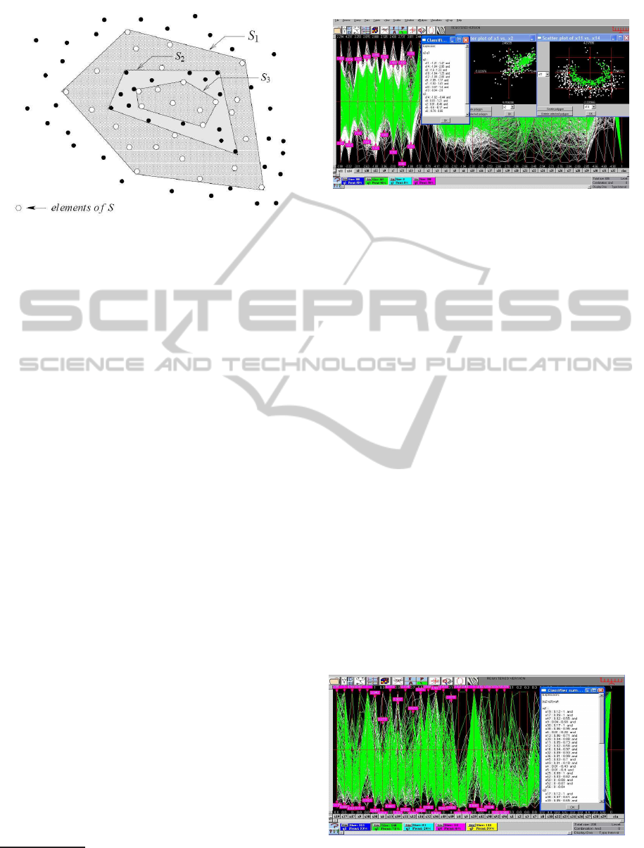
Figure 1: Construction of enclosure for the Nested Cavi-
ties algorithm. The first “wrapping” S
1
is the convex hull
of the points of S which also includes some points of P− S.
The second wrapping S
2
is the convex hull of these points
and it includes some points of S which are enclosed with
the third wrapping S
3
. To simplify the wrappings are shown
as convex hulls rather than as approximations. Here the se-
lected set is S = (S
1
− S
2
) ∪ (S
3
− S
4
) where S
4
=
/
0.
dropped and some points of S may be omitted (“false
negatives”), while some points of P− S are allowed
(“false positives”) in the hypersurface. The descrip-
tion of such a hypersurface provides a rule for iden-
tifying, within an acceptable error, the elements of S.
The use of Parallel Coordinates also enables visual-
ization of the rule.
At first the algorithm determines a tight upper
bound for the dimension R of S. For example, P may
be a 3-dimensional set of points but all point of S may
be on a plane; in which case S has dimension 2. Once
R is determined R variables out of the N are chosen
according to their predictive value and the construc-
tion process, schematically shown in Fig. 1, operates
only on these R selected variables. It is accomplished
by :
♦ use of a “wrapping” algorithm to enclose the
points of S in a hypersurface S
1
containing S and
typically also some points of P− S; so S ⊂ S
1
1
.
♦ the points in (P − S) ∩ S
1
are isolated and the
wrapping algorithm is applied to enclose them,
and usually also some points of S
1
, producing a
new hypersurface S
2
with S ⊃ (S
1
− S
2
),
♦♦ the points in S not included in S
1
− S
2
are next
marked for input to the wrapping algorithm, a
new hypersurface S
3
is produced containing these
points as well as some other points in P − (S
1
−
S
2
) resulting in S ⊂ (S
1
− S
2
) ∪ S
3
.
1
By S
j
⊂ S
k
it is meant that the set of points enclosed in
the hypersurface S
j
is contained in the set of points enclosed
by the hypersurface S
k
Figure 2: The dataset with 32 variables is shown in the
background. It has 2 categories whose points are differ-
encly colored. The table contains the explicit rule. The left
scatterplot shows the first two consecutive variables. The
classifier found that only 9 variables, whose ranges are in-
dicated by the downward and upward arrowheads on their
axis, are needed to describe the rule with a precision of 4%.
The plot of the right shows the two best predictors and the
separation achieved between the two categories.
♦ The process is repeated alternatively producing
upper and lower containment bounds for S; termi-
nation occurs when an error criterion is satisfied
or when convergence is not achieved.
The algorithm decomposes P into nested subsets,
hence the name Nested Cavities (abbr. NC) for the
classifier. The nested subsets are disjoint so they are
partitions of P. Basically, the “wrapping” algorithm
produces a convex-hull approximation; the techni-
cal details are not needed here. It turns out, that in
many cases using rectangular parallelopipeds for the
wrapping suffices. compared to those obtained by 22
other well-known classifiers (see (Inselberg and Avi-
dan, 2000)). The overall computational complexity is
O(N
2
|P|) where N is the number of variables and |P|
is the number of points in P
A dataset with 32 variables x
1
, x
2
, . . . , x
32
having 2
categories each having 300 points is chosen to exem-
Figure 3: Sonar dataset with 60 variables and 2 categories.
The NC classifier partitions the dataset into 3 nested sub-
sets indicated by the 3 rectangles, in middle of the lower
row, with 148, 51 and 14 items each. To improve the visual
clarity some of the variables (axes) not needed in the rule
were removed.
DATA2012-InternationalConferenceonDataTechnologiesandApplications
80

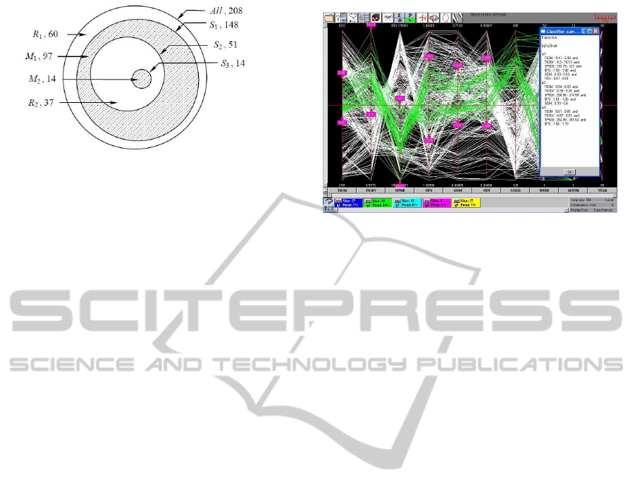
Figure 4: Schematic of the sonar dataset partition. The
S
i
are the nested subsets, R = R
1
∪ R
2
and the mines M =
M
1
∪ M
2
. Together with the notation is the number of items
contained in each subset.
plify the process. The NC classifier applied to cate-
gory 1 found that only the variables, ordered by their
predictive value, x
11
, x
14
, x
8
, x
10
, x
12
, x
9
, x
7
, x
23
, x
13
are
needed to specify the classification rule in only one
iteration and about 6% error. The second iteration in-
volves additionally x
2
, x
5
, x
6
reducing the error to 4%.
The result is shown in Fig. 2; the separation achieved
is striking.
Two error estimates are used: Train & Test and
Cross-correlation. When the rule involves several it-
erations an additional criterion is employed to avoid
overfiting. Namely, the rule error is traced iteration
by iterations and the process is stopped when the error
increases compared to the previous. As pointed out in
(Inselberg and Avidan, 2000), the rule obtained by the
NC classifier were applied to 4 bench-mark datasets
and were the most accurate compared to those ob-
tained by 22 other well known classifiers.
3 PARTIONING INTO
SUB-CATEGORIES
As one might expect things do not always work out
as nicely as for the example. The sonar dataset from
(UCI, 2012) has been a real classification challenge
with which we illustrate the new divide-and-conquer
idea. It has 60 variables, 208 observations and 2 cat-
egories 1 for Mines with 111 observations and 0 for
Rocks with 97 data points. Applying the NC classifier
partitions the dataset into 3 nested subsets S
1
, S
2
, S
3
,
with 148, 51 and 14 items respectively, The rule ob-
tained involves about 35 variables and an unaccept-
able high error of about 45%. The result, demarcat-
ing the nesting (by the rectangles in the lower row)
and showing some of the variables used in the rule is
shown in Fig. 3.
The schematic in Fig. 4 clarifies the partition of
the dataset into 4 disjoint sets, M
1
, M
2
for the mines
and R
1
, R
2
for the “rocks”. These are obtained by S
3
=
Figure 5: This is a financial dataset where subset corre-
sponding to the high-gold prices is selected. The classifi-
cation by NC partitions this subset into two (indicated by
the 2 and 4th rectangle in the lower row) as for the sonar
dataset.
M
2
, R
2
= S
2
− S
3
, M
1
= S
1
− S
2
and R
1
= All − S
1
where All stands for the full dataset. This is a very
useful insight into the structure of the dataset and mo-
tivates the idea. The bulk of the mines are in M
1
which has the higher values of the variables needed
to specify the rule. By contrast, the subset M
2
= S
3
is
a small “island”, having the smaller variable values,
surrounded by R
2
differs markedly from M
1
.
Consider R ∪ M
1
and apply the NC classifier.
A rule distinguishing M
1
from R is found needing
only 4 variables. Due to small size of M
1
the er-
ror estimates, with either cross-correlation or train-
and-test the number of “false-negatives” were high,
about 30%, though the “false-positives” were about
5% yielding a weighted average error of about 15%.
For another interesting comparison distinguishing M
1
from M, NC yields a rule with 5 variables and an 8%
average error. It is clearthat M
1
is easily distinguished
both from the “rocks” and the larger class of mines
M
1
.
This strongly suggests that there are two very dif-
ferent types of mines included in this dataset. To sum-
marize part of NC’s output, indicated by the rectan-
gles in the lower row of the figure, gives the decom-
position of the dataset into nested subsets. From these
one or more of the categories can be partitioned to
obtain a more accurate and simpler rule. While this
has been observed for some time it was only investi-
gated recently. Of course, the idea of partitioning is
inherent in classification which after all pertains to the
division of a dataset and differentiating between the
parts. While there is a lot of literature on partitions
in data mining, as we already pointed out, this spe-
cific method has apparently not been proposed. Such
a decomposition can clearly be automated and also
the classification of the new categories can be done in
GeometricDivideandConquerClassificationforHigh-dimensionalData
81

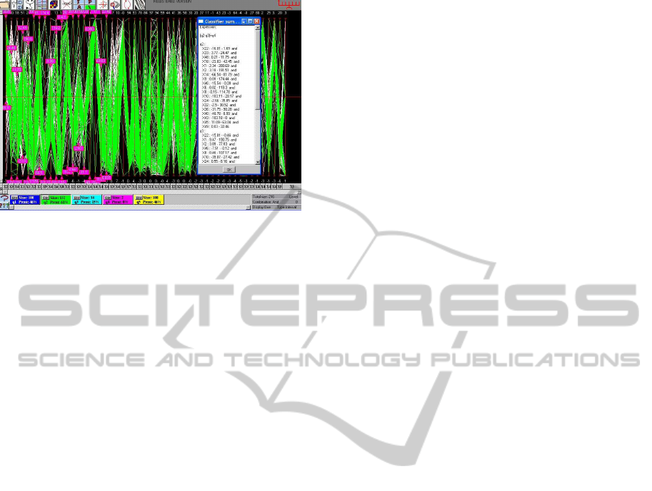
Figure 6: This a dataset with measurements pertaining to
ovarian cancer having 50 variables and 3 categories. Classi-
fication by NC of one category yields a complex and inaccu-
rate rule. It also partitions it into 2 sub-categories yielding
simpler and more precise rule. It also suggests that this type
of cancer has two different descriptions (morphologies).
parallel.
We have encountered similar situations with other
datasets. For the financial dataset shown in Fig. 5, the
data corresponding to a high price range for gold is the
selected subset. Classification with NC showed that
there are two different sets of conditions which cause
the price of gold to rise. These are better characterized
separately as for the sonar dataset. Interestingly, the
price of Yen is involved in one of the conditions but
not the other.
Another such example is shown in Fig. 6 for a
dataset with measurements on ovarian cancer having
50 variables and 3 of categories (types of cancer).
Classification of one category yielded a complex and
imprecise rule. However, it also showed a decompo-
sition into two sub-classes for which good rules were
obtained. Since different descriptors were involved
for each sub-class the thought arises that the cancer
types are really different. These examples are generic
of a common problem in classification, and for these
we offer a time-honored solution: divide and con-
quer.
REFERENCES
Fayad, U. M. Piatesky-Shapiro, G., Smyth, P., and Uthu-
rusamy, R. (1996). Advances in Knowledge Discov-
ery and Data Mining. AAAI/MIT Press, Cambridge
Mass.
Inselberg, A. (2009). Parallel Coordinates : VISUAL
Multidimensional Geometry and its Applications.
Springer, New York.
Inselberg, A. and Avidan, T. (2000). Classification and Vi-
sualization for High-Dimensional Data, in Proc. of
KDD, 370-4. ACM, New York.
Kugler, M. (2006). Divide-and-Conquer Large-Scale Sup-
port Vector Classification. Ph.D. Thesis, Dept. of
CSE, Nagoya Inst. of Tech.
Marchand, M. and Shawe-Taylor, J. (2002). The set cover-
ing machine. J. Mach. Learn. Res.
Mavroforakis, M., Sdralis, M., and Theodoridis, S. (2006).
A Novel SVM Geometric Algorithm based on Reduced
Convex Hulls. Pat. Rec. ICPR Inter. Conf. 564-568.
McBride, B. and Peterson, L. G. (2004). Blind Data Classi-
fication Using Hyper-Dimensional Convex Polytopes.
Proc. AAAI.
Murthy, S. and et al (1993). OC1: Randomized Induction
of Oblique Desicion Trees. AAAI.
UCI (2012). Machine Learning Database Repository at.
www.ics.uci.edu/ mlearn/MLRepository.html.
Xindowg, W. and et al (2008). Top 10 algorithms in data
mining. Knowl. Inf. Syst., 14:1–37.
DATA2012-InternationalConferenceonDataTechnologiesandApplications
82