Rate of Penetration Prediction and Optimization using Advances in

Artificial Neural Networks, a Comparative Study

Khoukhi Amar and Alarfaj Ibrahim

Systems Engineering Department, KFUPM, Dhahran, K.S.A.

Keywords: Prediction, Rate of Penetration, Regression, ANN, ELM, RBF.

Abstract: An important aspect of oil industry is rate of penetration (ROP) prediction. Many studies have been

implemented to predict it. Mainly, multiple regression and artificial neural network models were used. In

this paper, the objective is to compare the traditional multiple regression with two artificial intelligence

techniques; extreme learning machines (ELM) and radial basis function networks (RBF). ELM and RBF are

artificial neural network (ANNs) techniques. ANNs are cellular systems which can acquire, store, and

utilize experiential knowledge. The techniques are implemented using MATLAB function codes. For ELM,

the activation functions, number of hidden neurons, and number of data points in the training data set are

varied to find the best combination. Different input parameters of ELM give different results. The

comparison is made based on field data with no correction, then with weight on bit (WOB) correction, and

finally with interpolated WOB and rotary speed (RPM) correction. Seven input parameters are used for

ROP prediction. These are depth, bit weight, rotary speed, tooth wear, Reynolds number function, ECD and

pore gradient. The techniques are compared in terms of training time and accuracy, and testing time and

accuracy. Simulation experiments show that ELM gave the best results in terms of accuracy and processing

time.

1 INTRODUCTION

Cost efficiency in oil drilling projects becomes a

very important aspect nowadays. Efforts to predict

effects of drilling parameters and to optimize such a

cost have been widely done in many studies and

reports. These studies aim to increase the

performance and decrease the probability of

encountering problems. In most cases, drilling cost

is reduced by increasing drilling speed. This is

mainly done by maximizing the rate of penetration

(ROP). ROP depends on many other drilling

parameters. The relationship between drilling

parameters are studied to maximize ROP by finding

the optimum drilling parameters (Gidh et al., 2011);

(Bataee and Mohseni, 2011).

The prediction of ROP helps to select the best

input parameters to get the highest drilling rate with

the least cost. Thus, it has been the focus of many

researcher and oil companies. Research is still going

to find most accurate results. Therefore, it is

important to compare between different techniques

to choose the most accurate prediction.

On the other hand, the applications of

Computational Intelligence (CI) methods in

petroleum engineering have recently emerged as

powerful tools leading to a new generation of

computer aided analysis tools for practitioners,

scientists, and engineers working in several areas of

petroleum industry (Khoukhi, 2012); (Khoukhi et

al., 2011); (Khoukhi and Albukhitan, 2010);

(Motahhari et al., 2009); (Samuel et al., 2007). This

paper presents a comparative study between the

traditionally-used regression-based models with two

important artificial neural network techniques on the

rate of penetration prediction problem.

Currently, the available computing and

modelling techniques for ROP prediction implement

multiple regression models, operations research,

artificial neural networks (ANN), and simulation.

The parameters that affect ROP are difficult to

model. Different input parameters are used in

different studies. Weight on bit (WOB) and

rotational speed per minute (RPM) are the main

parameters that are used in most reported literature

(Motahhari et al., 2009); (Samuel et al., 2007);

(Bourgoyne and Young, 1974); (Eren, 2010).

Unfortunately, the models in the existing studies

647

Amar K. and Ibrahim A..

Rate of Penetration Prediction and Optimization using Advances in Artiﬁcial Neural Networks, a Comparative Study.

DOI: 10.5220/0004172506470652

In Proceedings of the 4th International Joint Conference on Computational Intelligence (NCTA-2012), pages 647-652

ISBN: 978-989-8565-33-4

 2012 SCITEPRESS (Science and Technology Publications, Lda.)

have some limitations. First, they did not consider

all possible input parameters, which most probably

result in lower accuracy of the results. Second, the

data prediction speed is low (Huang et al., 2011);

(Mark, 1996); (Paiaman et al., 2009); (Hamrick,

2011); (Sultan et al., 2002); (Rampersad et al.,

1994); (Abtahi et al., 2011).

The scope of this paper is to compare results

obtained by a multiple regression model to those

obtained using extreme learning machine (ELM) and

radial bases function networks (RBF) in terms of

accuracy and processing speed. ELM and RBF use

the concept of neural networks. The neurons learn

when fed with the data. In previous ELM

applications, neurons understand faster than other

artificial intelligence techniques (Huang et al.,

2006); (Huang, 2010); (Adrian, 1996). Carefully

evaluating input parameters is crucial for the model

to be fast. The output data will be compared with

actual oil and gas data. Recently, a prime study

showed the significant add on value of ANN to ROP

prediction (Moran et al., 2010); (Awasthi and

Ankur, 2008).

The main contribution of this paper as compared

to the previous studies is that it investigates ELM

and RBF

models, which were not used before in

ROP prediction. Moreover, it provides effective

choices of ELM structural parameters and activation

functions for a better ELM prediction. Furthermore,

it shows the best of three models (ELM, RBF,

regression) to help decision makers.

2 METHODOLOGY

The methodology followed is to implement each

technique with different structural parameters, and

activation functions, number of hidden nodes, and

then compare the best results from each technique

with the other techniques.

Both ELM and RBF are single hidden layer

feedforward networks (SLFN). These particular

techniques were chosen for several reasons. ELM

and RBF usually give very good results in other

fields as compared e.g. to multi-layer perceptron.

Also, they are new techniques in the field of ROP

prediction, which adds new information to the field.

Regarding regression, it is widely used in ROP

prediction. Therefore, it is important to show

whether changing the common technique

(regression) to a new technique is justifiable or not.

3 IMPLEMENTATION

3.1 Input / Output Data

Mainly, the methodology was implemented to

provide comparable results. The same dataset is

inputted to ELM and RBF. In the beginning of this

work an initial published data by Bourgoyne and

Young (1974) was implemented.

Seven input drilling parameters were used in the

study. These are depth, bit weight, rotary speed,

tooth wear, Reynolds number function, ECD and

pore gradient. At a second stage, the used dataset for

these inputs were those used in Eren’s (2010) as to

provide a fair comparison of the proposed models

with the multiple regression model. The outputs

from the three models are compared. The

comparison is based on training time and accuracy

and testing time and accuracy.

3.2 Computer Codes

Developed by Dr. Huang, a MATLAB function code

is used to process data using ELM. The code was

run into a loop one thousand times and then an

average is taken to avoid variations due to random

initializations. The parameters of ELM are changed

and compared to find the best combination. The

changed parameters are the number of hidden

neurons, the activation function, and the

stratification percentage of training data.

Regarding RBF, a MATLAB built in function

(newrb) is used to process the data (Mathworks,

2007 a, b). The target training accuracy and

percentage of training data are also changed to find

the best combination.

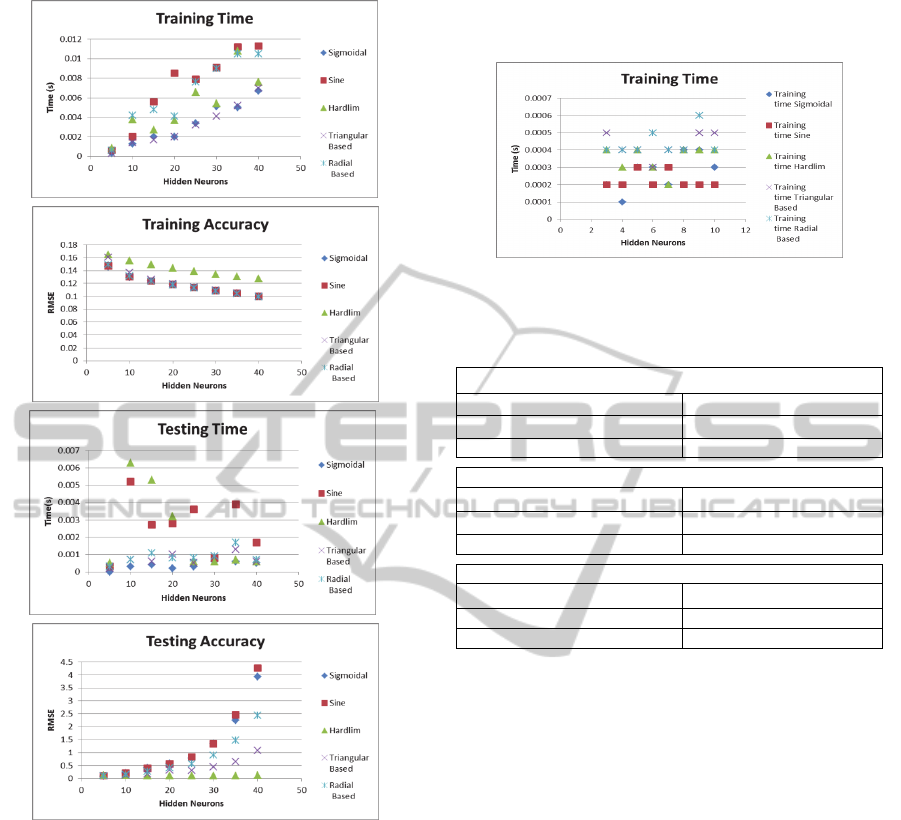
3.3 Simulation Results

The preliminary simulation experiments are very

encouraging. Each technique gave different results

in terms of comparison criteria. The results are being

shown for each element. For ELM, it was found that,

as in Fig. 1, the time and accuracy are better when

the number of hidden neurons is 5. Therefore, values

around 5 were taken for the number of hidden

neurons (3 to 10).

For RBF, the goal (mean square error MSE) will

be taken to be either 6400 ft

or 4900 ft

which

is, respectively, similar to and better than what ELM

gave. Also, the spread parameter is 20,30,40,50, or

100. Table 1 shows a sample of RBF results of

Accuracy and Training Time(s) vs. Spread

Parameter.

IJCCI2012-InternationalJointConferenceonComputationalIntelligence

648

Figure 1: a)Training Time, b) training accuracy, c) testing

time and d) testing accuracy, vs. No. of hidden neurons

(5to50).

4 TRAINING TIME

With ELM, as shown in Fig. 2, the training time is

not affected by the small changes in the number of

hidden nodes. The small random variations are due

to processor variability. Moreover, comparing

among the different activation functions, one can see

that it requires more time to train a set using

triangular and radial basis function than using the

other three activation functions.

RBF requires more training time than ELM does.

It requires almost the same training time at the

values of MSE used. Furthermore, it does not seem

to be affected by the change of the spread parameter.

A sample of the results is shown in Table 1.

Figure 2: ELM training time.

Table 1: RBF accuracy and training time(s) vs. spread

parameter.

Spread = 20

Target training MSE Training Time(s)

4900 0.156

6400 0.156

Spread = 40

Target training Acc. Training Time(s)

4900 0.1404

6400 0.156

Spread = 100

Target training Acc. Training Time(s)

4900 0.1248

6400 0.156

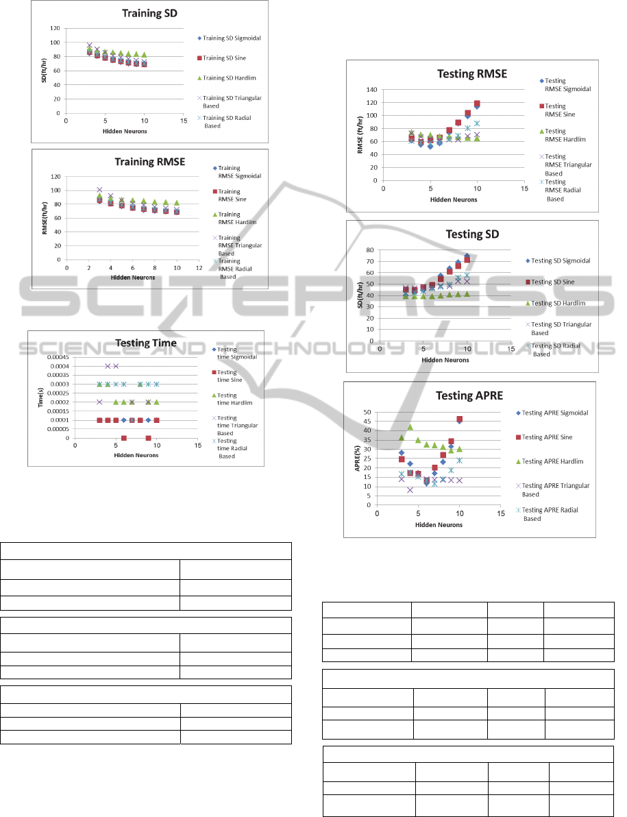
4.1 Training Accuracy

Using root mean squared error (RMSE) and standard

deviation (SD), ELM gave relatively more accurate

training results. The accuracy gets better with

increasing hidden neurons. Hardlim function

provides the least accurate results. Other functions

give the very close RMSE. The results can be

deduced from Fig. 3 which shows the RMSE and SD

of the data in ft/hr.

RBF training accuracy is set to be either

mse=6400 or mse=4900 ft

/hr

. However the choice

affects the time and accuracy of training and testing.

4.2 Testing Time

Testing time for ELM seems random and not

affected by the number of hidden neurons. The

sigmoid and sine functions gave the best results and

hardlim, triangular basis, and radial basis gave the

worst. Results are shown in Fig. 4.

RBF gave higher testing time than ELM. Testing

Time is not affected by the choice of goal training

accuracy n or the value of the spread, as shown in

Table 2.

RateofPenetrationPredictionandOptimizationusingAdvancesinArtificialNeuralNetworks,aComparativeStudy

649

Figure 3: ELM Training Accuracy, a) RMSE, b)SD.

Figure 4: ELM testing time vs. No. of hidden neurons.

Table 2: RBF accuracy vs. spread parameter testing time

data.

Spread = 20

Target training Acc. Testing Time (s)

4900 0.1092

6400 0.078

Spread =40

Target training Acc. Testing Time (s)

4900 0.1092

6400 0.0936

Spread= 100

Target training Acc. Testing Time (s)

4900 0.1248

6400 0.0936

4.3 Testing Accuracy

ELM's testing RMSE, SD, and APRE have minima

at different number of hidden nodes at each

activation function. Fig. 5 displays these minima.

RBF testing was not accurate, when training

target MSE is chosen low and very good when it is

chosen close to ELM's training accuracy, as can be

seen in Table 3.

c c

Figure 5: ELM testing accuracy.

Table 3: RBF testing accuracy.

Spread = 20

arget training Acc. Testing RMSE Testing SD Testing APRE

4900 154.8288 104.8767 82.81

6400 34.996 34.9756 9.6

Spread =40

Target training Acc. Testing RMSE Testing SD Testing APRE

4900 129.375 89.5038 54.21

6400 35.0248 35.0017 9.63

Spread=100

Target training Acc. Testing RMSE Testing SD Testing APRE

4900 144.3341 101.6538 70.73

6400 35.0328 35.009 9.63

IJCCI2012-InternationalJointConferenceonComputationalIntelligence

650

4.4 Discussion

The methods’ accuracies are compared in terms of

RMSE, standard deviation SD, and absolute percent

relative error (APRE). The regression gave for no

correction, average APRE is 111%, RMSE is 210.39

ft/hr and SD is 179.89 ft/hr. For WOB correction,

the average APRE is 85%, RMSE is 133.73ft/hr and

SD is 107.18 ft/hr. For interpolated correction,

average APRE is 30%, RMSE is 57.29 ft/hr and SD

is 57.25 ft/hr. Therefore, the interpolated correction

are compared with the other techniques and the data

plugged in ELM and RBF models are those of the

interpolated corrected.

For ELM, we see each activation function

separately. From Fig. 5, it can be seen that the most

accurate results are at sigmoidal with 5 hidden

neurons. Table 3 shows that the most accurate

method of implementing RBF is with MSE = 6400

/hr

and spread = 20. Therefore, we take this

combination as the candidate of comparison. Table 4

shows the comparison among the techniques in

terms of testing accuracies.

Comparing the results above, we can see that

RBF is the most accurate technique. However, ELM

is the fastest. Therefore, depending on the objective,

a decision can be made.

Table 4: Comparison of testing accuracies.

technique

ELM RBF Regression

criterion

RMSE(ft/hr) 51.9716 34.996 37.36152

SD(ft/hr) 44.405 34.9756 64.71206

APRE 17.13% 9.6% 33%

5 CONCLUSIONS

This paper has shown a comparison among ELM,

RBF, and a multiple regression model for ROP

Prediction. The professionals and decision makers

are advised, according to the results of this study, to

choose RBF as the ROP prediction technique.

However, if processing speed is more important, the

decision makers might want to use ELM. Additional

ANN techniques can be used in development of this

study. Some of them are being implemented in an

ongoing work.

ACKNOWLEDGEMENTS

The authors would like to thank KACST for

supporting this work under grant: KACST-OIL-AR-

30-258-2012, and Dr. Tuna Eren, for providing real

time data and regression models. Mr. Alarfaj gives

special thanks to KFUPM and Systems Engineering

Department for offering the SE 439 course on

undergraduate research.

REFERENCES

Abtahi A., Butt S., and Molgaard, J., and Arvani F., 2011.

“Bit Wear Analysis and Optimization for Vibration

Assisted Rotary Drilling

) VARD (using Impregnated

Diamond Bits”, Memorial University of

Newfoundland, St. John’s, NL, Canada.

Adrian G. Bors 1996. “Introduction to the Radial Basis

Function (RBF) Networks”, University of York.

Available: www-sers.cs.york.ac.uk/adrian/Papers/

Others/OSEE01.pdf>.

Awasthi, Ankur 2008. “Intelligent oilfield operations with

application to drilling and production of hydrocarbon

wells”, University of Houston, 2008, 370p.

Bataee M., & Mohseni, S., 2011. “Application of artificial

intelligent systems in ROP optimization: A case study

in Shadegan oil field”. SPE Middle East

Unconventional Gas Conference and Exhibition

2011.

Bourgoyne A.T. Jr., Young F.S., 1974 “A Multiple

Regression Approach to Optimal Drilling and

Abnormal Pressure Detection”, SPE 4238, August

1974.Available: ttp://www.onepetro.org/mslib/servlet/

onepetropreview?id=00004238>.

Eren Tuna, 2010. “Real-Time-Optimization Of Drilling

Parameters During Drilling Operations Dissertation”

PhD

Technical University of the Middle East, Turkey.

“Getting Started with Matlab 7” www.mathworks.com

(2007).

Gidh Yashodhan, Ibrahim Hani, Purwanto Arifin, and Bits

smith, 2011. “Real-time drilling parameter

optimization system increases ROP by

predicting/managing bit wear”. SPE Digital Energy

conference and Exhibition, 2011.

Hamrick, Todd Robert, 2011. “Optimization of Operating

Parameters for Minimum Mechanical Specific Energy

in Drilling”, West Virginia University, 148 p.

Huang, Guang-Bin, Wang, Dian Hui, and Lan, Yuan,

2011. “Extreme learning machines: a survey”, Int. J.

Mach. Learn. & Cyber. (2011) 2:107–122.

Huang, Guang-Bin, 2010. “Extreme Learning Machine:

Learning Without Iterative Tuning”, Available:

http://www.extreme-learning-machines.org/.

Huang, Guang-Bin, Zhu, Qin-Yu, Siew, Chee-Kheong,

2006. “Extreme learning machine: Theory and

applications”, SienceDirect.

http://www.mathworks.com/help/toolbox/nnet/ref/newrb.h

tml.

Khoukhi A., 2012. “Hybrid soft computing systems for

reservoir PVT properties prediction”, Computers and

Geosciences, Elsevier, vol. 44, p: 109–119 2012.

RateofPenetrationPredictionandOptimizationusingAdvancesinArtificialNeuralNetworks,aComparativeStudy

651

Khoukhi A., Oloso M., Abdulraheem A., El-Shafei M.,

Al-Majed A., 2011. “Support Vector Machines and

Functional Networks for Viscosity and Gas/oil Ratio

Curves Prediction”, Int’l Journal of Computational

Intelligence and Applications vol. 10, No. 3, Oct 2011,

pp: 269–293.

Khoukhi A., Albukhitan S., 2010. “A Data Driven Genetic

Neuro Fuzzy System to PVT Properties Prediction”,

NAFIPS10, Toronto, Canada. 12-14 July 2010.

Mark J. L. Orr 1996. “Introduction to Radial Basis

Function Network”, Center of Cognitive Science,

University of Edinburg, April, 1996. Available:

http://www.anc.ed.ac.uk/rbf/intro/intro.html.

Moran David, Ibrahim Hani, Purwanto Arifin, Smith

International and Jerry Osmond, 2010. “Sophisticated

ROP Prediction Technologies Based on Neural

Networks Delivers Accurate Drill Time Result”, SPE

Asia Pacific Drilling Technology Conference and

Exhibition, 2010.

Motahhari H.R., Hareland G., Nyqaard R., and Bond B.,

2009. “Method of optimizing motor and bit

performance for maximum ROP”, Journal of

Canadian Petroleum Technology, 2009.

Paiaman A. M., Al-Askari M. K. Ghassem, Salmani B, Al-

Anazi, B. D. and Masihi M. 2009. “Effect of Drilling

Fluid Properties on Rate of Penetration”, NAFTA 60

(3) 129-134 (2009).

Rampersad, P.R., Hareland, G.; and Boonyapaluk, P.,

1994. “Drilling Optimization Using Drilling Data and

Available Technology”, SPE Latin

America/Caribbean Petroleum Engineering

Conference, 27-29 April 1994, Buenos Aires,

Argentina.

Samuel G., Robello, Azar, Jamal J., 2007. “Drilling

Engineering”, PennWell Books, 486p.

Sultan, Mir Asif, Al-Kaabi, Abdulaziz U, 2002.

“Application of Neural Network to the Determination

of Well-Test Interpretation Model for Horizontal

Wells”, SPE Asia Pacific Oil and Gas Conference and

Exhibition, 8-10 October 2002, Melbourne, Australia.

IJCCI2012-InternationalJointConferenceonComputationalIntelligence

652