BISTATIC SYNTHETIC APERTURE RADAR TECHNOLOGY -
TOPOLOGIES AND APPLICATIONS
Andon Dimitrov Lazarov
CITS, Bourgas Free University,62 San Stefano Str. Bourgas, Bulgaria
Keywords: Bistatic Synthetic Aperture Radar, Bistatic Forwar Scattering Inverse Synthetic Aperture Radar .
Abstract: Bistatic Synthetic Aperture Radar (BSAR) and Bistatic Forward Inverse Synthetic Aperture Radar
(BFISAR) concepts are considered. Different BSAR topologies with transmitter of opportunity, stationary
receiver with moving target are analyzed. Forward scattering RCS is defined. Mathematical models of
BSAR and BFISAR signals and image reconstruction algorithms are presented. Results of numerical
experiment are discussed.
1 INTRODUCTION
Bistatic synthetic aperture radar (BSAR) technique
is under intensive research activities over the last ten
years. It makes an impact on the progress in
synthetic aperture radar (SAR) and inverse synthetic
aperture radar (ISAR) technologies and meets strong
requirements for the further enhancement of
microwave remote sensing systems. It is expected
that the implementation of BSAR concept in ISAR
will enlarge the area of application and improve
substantially the functionality of imaging radars.
Bistatic concept in SAR for Earth observation is
analyzed in (Moccia A., 2002). Prospective and
problems in space-surface BSAR are addressed in
(Cherniakov M., 2002) and BSAR with application
to moving target detection is described in
(Whitewood A., 2003). Several BSAR techniques
for image reconstruction have been proposed that
provide effective tools for radar imaging of
cooperative targets (D’Aria D., 2004). Effects of
bistatic configurations on ISAR imaging have been
largely investigated in (Martorella M., 2007).
2 BISTATIC SYNTHETIC
APERTURE RADAR
CONFIGURATIONS
2.1 Bistatic Radar Geometry
Bistatic radar geometry comprises a transmitter,
located in point A, a receiver located in point B, and
target located in point T (Fig. 1). Denote θ as a
bistatic angle, L = AB as a baseline, and Δ
R
as range
resolution
Figure 1: Bistatic radar geometry
Contours of constant bistatic range are ellipses with
transmitter and receiver as two foci. The following
equations can be written
R
T
(t) + R
R
(t) = L + n.Δ
R
,
(1)
)()(2
)()(
cos
222
tRtR
LtRtR
TT
RT
−+
=θ
, (2)
where n = 0,1,2, ….is the number of an isorange
ellipse. The number n = 0 corresponds to zero range
resolution on baseline L.
3
Lazarov A.
BISTATIC SYNTHETIC APERTURE RADAR TECHNOLOGY TOPOLOGIES AND APPLICATIONS.
DOI: 10.5220/0005413100030013
In Proceedings of the First International Conference on Telecommunications and Remote Sensing (ICTRS 2012), pages 3-13
ISBN: 978-989-8565-28-0
Copyright
c
 2012 by SCITEPRESS – Science and Technology Publications, Lda. All rights reserved

2.2 Bistatic Radar Equation
Bistatic radar equation represents signal-to-noise
ratio as a function of parameters of electromagnetic
propagation, radar and target, i.e.
BFkTRR
LFFGGP
P
P
RT
pBRTRTT
N
R
0
223
222
)4(
.
π
σλ
=
(3)
where P
R
- receiver power; P
N
- noise power; R
T
-
distance from the transmitter to the target; R
R
-
distance from the receiver to the target σ
B
- bistatic
radar cross − section of the target; G
T
- transmitter
gain; G
R
-receiver gain; -pattern propagation
factor for the transmitter-to-target-path; - pattern
propagation factor for the target-to-receiver path; k -
Boltzmann's constant; λ -wavelength; F – Figure of
merit; T
2
T
F
2
R
F
0
-noise temperature.
The constant detection range is defined by
that describes ovals of Cassini around
transmitter and receiver points (Fig. 2).
const=
RT
RR
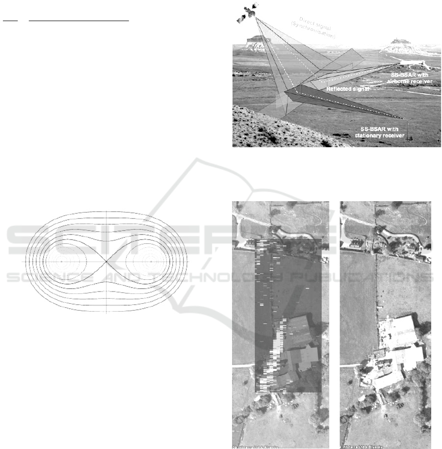
Figure 2: Ovals of Cassini
2.3 BSAR for Local Area Monitoring
A new topology of BSAR with non cooperative
transmitter is presented in (Cherniakov M., 2009,).
The topology includes Global Navigation Satellite
Systems (GNSS) as transmitters of opportunity and a
stationary receiver placed on the ground. It is a
system for local area monitoring. BSAR with non
cooperative transmitter is a sub-class class of bistatic
SAR systems that comprises a spaceborne
transmitter, and a receiver located on or near the
Earth’s surface (Fig. 3). As a sub-class of BSAR, it
encompasses a variety of system topologies. Any
communication or Global Positioning System (GPS)
satellite can be used as a noncooperative transmitter
while the receiver could be airborne, onboard a
ground moving vehicle or stationary on the ground.
Different BSAR configurations have been
considered (Whitewood A., 2007). It has been the
investigated passive BSAR, with GNSS as
transmitters of opportunity (such as GPS,
GLONASS and Galileo) and an airborne receiver
(Antoniou M., 2009).
Figure 3: BSAR topologies
An image with a Galileo satellite as a transmitter and
a ground moving vehicle as a receiver has been
obtained (Fig. 4)
Figure 4: BSAR image of a building with Galileo as the
transmitter and a moving ground vehicle as the receiver
superimposed on a satellite optical photograph (a), optical
photograph (b).
The BSAR topology with a satellite transmitter has
military applications based on the potential of the
system to operate covertly due to its passive nature,
its ability to provide constant monitoring of any
First International Conference on Telecommunications and Remote Sensing
4

remote region on the Earth due to the global
coverage of the GNSS satellites. It is important to
investigate whether this system can be implemented,
to consider satellite availability, to identify whether
fast update rates for change detection can be
achieved, to examine basic radar functionality,
which involves calculations on integration time,
resolution and power budget.
2.3.1 Satellite availability and observation
time
Satellite availability can help define the available
observation time for imaging and the update rates
for change detection. It means the number of
satellites simultaneously visible at any point in the
world and the position of each satellite with respect
to the receiver to be defined. An optimal satellite can
be used for imaging to minimize degradation in the
system’s range resolution due to the large bistatic
angle (Willis N.J., 2007). It was found that
approximately 6-8 satellites are simultaneously
visible at a particular point on the Earth, at any time
(Zuo R., 2007). Another issue is the achievable
observation time. This is defined as the amount of
time that a target on the Earth is within the beam of
a satellite (assuming it is always within the beam of
the receiver). Even though the beam of the GNSS
satellites covers a large part of the Earth’s surface,
the observation time may vary significantly from
one satellite to another because of their position with
respect to the target. Fig. 5 shows results of
Keplerian modelling to define observation time
versus satellite number (Cherniakov M., 2009).
Figure 5: Observation time versus satellite number
according to Keplerian modeling
The figure shows that within an interval of one day,
22 satellites are visible in a nearly quasi-monostatic
mode, with observation times varying from 12
minutes to 3 hours. These values allow for very long
integration times due to satellites’ wide beam. It
provides fine azimuth resolutions, and enhances
power budget of the system.
2.3.2 Azimuth resolution
GNSS satellites on MEO with ranges of 23000 km
from the Earth, orbital speeds 4 km/s, and long
observation time provide a significant improvement
in azimuth resolution. The maximum azimuth
resolution that can be achieved for data in Fig. 5 is
shown in Fig. 6. The resolution is calculated through
Doppler bandwidth of the associated GPS azimuth
signals, and dividing with the average speed of the
satellite towards the observed target. The figure
shows that extremely high azimuth resolutions can
be potentially achieved if the full observation time is
processed. Even for an observation time of 12
minutes the resolution is reasonable.
Figure 6: Potential azimuth resolution for SS-BSAR
with stationary receiver.
2.3.3 Power Budget
Since GNSS satellites exhibit a low signal power
density on the Earth’s surface, long observation
times will essentially enhance the signal-to-noise
ratio (SNR) at the output of the image formation
algorithm used. Assuming full target signal
compression in both range and azimuth, the SNR
can be derived as
u
T
T
kTR
GP
SNR
obs
sR
RD
Δ
π
σλ
=
int
22
2
)4(
(4)
where P
D
is the signal power density of the GNSS
satellites on the Earth, G
R
is the gain of the receiving
antenna, λ is the radar wavelength, σ is the target
radar cross section, R
R
is the receiver-to-target range,
k is Boltzmann’s constant, T
S
is the receiver noise
temperature, T
int
is the integration time in the range
direction (equal to the length of the transmitted
Bistatic Synthetic Aperture Radar Technology - Topologies and Applications
5

GNSS code sequence), T
obs
is the observation time
and Δu is the azimuth sample spacing.
The challenge in this task is the long integration
time, over which the trajectory of the satellite can no
longer be considered a straight line. It can be seen in
Fig. 7, where the trajectory of one of the satellites in
our previous example (Fig. 5, satellite number 14)
has been plotted in 3-D space.
Figure 7: Example of a satellite trajectory over a long
observation time (satellite number 14)
2.3.4 Signal synchronization in BSAR based
on GLONASS satellite emission
BSAR coherent signal processing requires
synchronization between the transmitter and the
receiver (Fig. 8) (R.Saini, 2009).
Figure 8: BSAR topolody with synchronization.
Fig. 9 illustrates block diagram of the structure of
GLONASS signals transmitted in the L
1
frequency
band. The C/A and P-code signals are in phase
quadrature. The C/A code rate is 511 KHz and the
code period is 1 msec. The C/A code sequence is
added (mod 2) to a 100 Hz navigation message. The
P-code has a chip rate of 5.11 MHz and is a
truncated M-sequence repeated every 1 sec. The
navigation message on the P-code has a clock rate of
50 Hz. The P-code is used for the purpose of
imaging, as it provides a reasonable range resolution
of about 30m (quasi-bistatic case) and is no longer
encrypted. It is worth mentioning that utilization of a
GALILEO satellite E
5
signal (20-50 MHz
bandwidth) would improve the range resolution to
about 3-8 m.
Figure 9: Signal structure of GLONASS
Usually in a radar signal processor, the range
compression consists of a correlation of the radar
channel signal with the heterodyne channel signal
delayed for each range resolution cell in the multi-
channel correlator (Fig. 10).
Figure 10: Heterodyne channel with omny antenna (a) and
multi-channel correlator (b).
It was demonstrated that for GLONASS signal it is
not possible to directly correlate the heterodyne
channel with the radar channel. The signal received
from the GLONASS satellite is a superposition of
the C/A code and P-code signals, the spectra of
which overlap; the P-code (5.11 MHz bandwidth) is
used for the purpose of imaging. If the heterodyne
First International Conference on Telecommunications and Remote Sensing
6

channel is directly correlated with the radar channel,
the P-code will be masked by the C/A code at the
output of the correlator. The bandwidth of the C/A
code is only one-tenth that of the P-code but even if
the C/A code of the desired satellite signal is filtered
out in the heterodyne channel, the signal correlation
properties are degraded by the C/A codes of
interfering satellites. It was demonstrated that, if the
radar channel signal is correlated with a locally
generated signal containing only the P-code, the
effect of the C/A code could be suppressed.
However this technique needs navigation message
decoding which, in turn, requires P-code
synchronization. Fig. 11 illustrates a range
compression algorithm. Fig. 12 shows a simplified
synchronization block diagram.
Figure 11: Range compression algorithm.
Figure 12: Synchronization block diagram
A synchronization block diagram is presented in Fig.
12. The P-code has a better delay tracking accuracy
due to its wider signal bandwidth compared to the
C/A code. The synchronization algorithm is based
on a conventional delay locked loop, and consists of:
- Doppler extraction using the C/A code and
applying conventional phase locked loops.
- Removing the frequency shift from the received P-
code by extracting frequency variation.
- Synchronize the locally generated P-code to the
Doppler-stripped P-code.
- Decode the navigation message signal by
synchronized P-code, fraction of a chip. Once the
incoming P-code has been acquired, tracking, or fine
synchronization, takes place.
2.4 Bistatic generalized inverse
synthetic aperture radar
Consider geometry of BSAR scenario with a moving
target illuminated by GPS waveform and a
stationary GPS receiver. It refers to geometry of
Generalized Inverse Synthetic Aperture Radar
(GISAR) and Bistatic Synthetic Aperture Radar
(BSAR) and regards as Bistatic Generalized Inverse
Synthetic Aperture Radar (BGISAR). The problem
posed is to describe the discrete geometry of
BGISAR scenario and based on it to derive a
mathematical model of a BGISAR signal (Lazarov
A., 2011).
2.4.1 BGISAR Scenario
BGISAR scenario is illustrated in Fig. 13 where
GPS transmitter, receiver (located on the land
surface) and a target are all situated in Oxyz, where
is the current position vector of the
transmitter in discrete time instant p, is the
current position vector of the mass center of the
target, is the stationary position vector of the
receiver. The target presented as an assembly of
point scatterers is depicted in Cartesian coordinate
system OXYZ, where is the position vector of
the ijkth point scatterer.
)( p
s
R
)(
'00
pR
r
R
ijk
R
Figure 13: BGISAR geometry
In Fig. 13: - the position vector of the
target’s mass center with respect to the transmitter,
- The position vector of the target’s mass
)(
'0
p
s
R
)(
'0
p
r
R
Bistatic Synthetic Aperture Radar Technology - Topologies and Applications
7

center with respect to the receiver, - the
position vector of the ijkth point scatterer with
respect to the transmitter, - the position
vector of the ijkth point scatterer with respect to the
receive, ΔX, ΔY, ΔZ – dimensions of the resolution
cell.
)( p
ijk
s
R
)( p
ijk
s
R
The round trip distance from GPS transmitter to the
target and GPS receiver is defined by
)()()( pppR
ijk
r
ijk
s
ijk
RR +=
.
(5)
The deterministic component of the BGISAR signal,
reflected by all point scatterers of the object for
every
p
th GPS C/A pulse train has the form
∑
⎭
⎬
⎫
⎩
⎨
⎧
π+
−ω−
=
ijk
ijk
ijkijk
tb
pttj
pTatpS
)](
))(([
)]([),( exprect
(6)
where
T
ptt
pT
ijk
ijk
)(
)(
−
=
is the time parameter
λπ=ω /2 c is the angular frequency, m/s
is the velocity of the light, is the binary
parameter of the C/A phase code modulated pulse
train, defined by coefficients of two Gold
polynomials, is the reflective coefficient of the
ijkth point scatterer, three-dimensional (3-D) image
function; is the time duration of the C/A phase
code,
8
10.3=c
)(tb
ijk
a
T
c
pR
pt
ijk
ijk
)(
)( =
is the round trip delay to
th point scatterer;
ijk Tkptt
ijk
Δ
−
+= )1()(
min
,
is the time duration of the phase segment, k is
the current number of segment,
TΔ
1023/
=
Δ= TTK
is the full number of segments of the C/A phase
code, is the relative dimension of the target.
The image extraction procedure comprises
1. Phase correction,
)(().,(
ˆ
),(
~
pjkpSkpS Φ= exp ,
2. Range compression by cross-
correlation,
,
∑
Δ+−π=
−+
=
1
ˆ
ˆ
)])1
ˆ
(([),(
~
)
ˆ
,
ˆ
(
~
Kk
kk
TkkbjkpSkpS exp
3. Azimuth compression by Fourier transform,
∑
⎭
⎬
⎫
⎩
⎨
⎧
⎥
⎦
⎤
⎢
⎣
⎡
π
=
= Np
ijk
pp
N
jkpSkpa
,1
ˆ
2
)
ˆ
,(
~
)
ˆ
,
ˆ
( exp
.
2.4.2 BGISAR numerical experiment
A numerical experiment was carried out to verify the
geometry and 3-D model of BGISAR signal with
GPS C/A code phase modulation and to prove the
correctness of developed digital signal image
reconstruction procedure. It is assumed that the
target, a flying helicopter is moving rectilinearly in a
3-D Cartesian coordinate system of
observation . GPS transmitter emits a C/A
code train. GPS satellite velocity: m/s.
Coordinates of the stationary GPS receiver:
m, m and m. The trajectory
parameters of the target: velocity m/s;
guiding angles. Parameters of the GPS C/A pulse
trains: wavelength m (carrier
frequency Hz), registration time
interval s, GPS C/A code PRF 1.023
MHz and respective time duration of the segment of
the C/A pulse s, time duration of
GPS C/A code s; full number of GPS C/A
pulses
Oxyz
206,3819=v
55=
r
x
45=
r
y
30=
r
z
80=V
2
10.1,19
−
=λ
9
10.57.1=f
3
10.2,2
−
=
p
T
6
10.9775.0
−
=ΔT
3
10
−
=T
1023
=
K , number of transmitted GPS C/A
code trains during aperture synthesis . In
Fig. 2 results are presented.
1024=N
(a) (b)
Figure 14. BGISAR signal processing stages: real (a) and
imaginary (b) parts, range compressed by correlation and
azimuth compressed by Fourier transform.
(a) (b)
First International Conference on Telecommunications and Remote Sensing
8

Figure 15. Original image of helicopter (a) BGISAR
image of helicopter (b)
3 BISTATIC FORWARD
SCATTERING RADAR
CONFIGURATIONS
3.1 Bistatic forward scattering radar
processing
Bistatic forward scattering radar (BFSR) is a sub-
class of bistatic radars, with a moving target and
bistatic angle between transmitter-target-receiver
close to 180
0
. The received signals are formed by
diffraction of the emitted electromagnetic waves.
The target can be considered as a secondary antenna
which has the target’s silhouette and with gain,
defined by the target radar cross-section (RCS)
which is independent from the target material. Such
systems can be used for stealth targets detection.
3.1.1 BFSR Scenario
Consider a BFSR scheme using CW signals for
situation awareness that includes a transmitter T and
receiver R situated on the ground or see surface and
a target with distances transmitter-target R
T
(t) and
target-receiver R
R
(t), and bistatic angle θ(t) (Fig.
16). Targets (humans or vehicles) are moving across
the transmitter-receiver baseline. A signature of a
moving target is received at the background of
clutter, noise and possibly interference.
Figure 16: BFSR scenario.
The deterministic signal at the input of the receiving
antenna is given by the sum of the direct transmitter-
receiver (leakage) signal and the signal reflected
from the target. The leakage signal is much stronger
than the signal from the target which can be
separated based on the Doppler signature induced by
displacement of the target.
3.1.2 BFSR signal processing and parameter
estimation
Signature processing includes signal compression
and target resolution by maximization of signal-to-
noise ratio (SNR) as the target signature could be
buried under noise at longer baselines (Cheng Hu,
2008).
Let target’s speed be a parameter estimated on the
baseline. Assume that the signal is corrupted only by
additive white Gaussian noise. SNR maximization is
realized by correlating the received signal
with a reference function , complex conjugated
of the target signature itself. The correlation process
is described by the equation
)(tS
T
)(
0
tS
∫
τ−=τ
−
2
2
0
)()()(
T
T
T
dttStSS
(7)
where T is the coherent processing interval,
τ
is the
correlation displacement.
This process is known as matched filtering, and
referred to as optimal signal processing algorithm. If
the reference function has a rectangular envelop, the
signal processing is quasi optimal.
Figure 17: Signature compression by optimal and quasi
optimal processing algorithms.
Compressed signatures for a single target obtain by
optimal and quasi optimal processing algorithms are
presented in Fig. 17.
3.2 BFSR radar cross section estimation
BFSR concept can be applied in monitoring and
protecting coast lines and off shore territories. Using
a chain of buoys, located on the sea surface and
equipped with FSR transceivers, schematically
shown in Fig. 18 (Liam Daniel, 2008).
Bistatic Synthetic Aperture Radar Technology - Topologies and Applications
9

Figure 18: A chain of buoys, located on the sea surface
and equipped with FSR transceivers
Objects crossing the baselines connecting adjacent
transceiver buoys could be detected through analysis
of their Doppler signature. Small targets with low
radar reflectivity such as jet-skis, inflatable boats
and swimmers could be detected.
BFSR RCS can be defined through optical
approximation: BFSR RCS of a complex object is
reduced to the radiation pattern of the silhouette
shape of that object (black body approximation), and
finding of the radiation pattern of this silhouette’s
uniformly (planar) illuminated complimentary plane
aperture (Babinet’s principle) (Fig. 19) (Daniel L.,
2008).
Figure 19 Figure: 20
Figure 19: Scatter from a complex object (a), reduced to
scatter from a plane shape (b), further reduced to
diffraction from an aperture (c).
Figure 20: Aperture projections in plane perpendicular to
wave propagation vector and (b) angular definitions for
analytic RCS (8).
In the direct forward scatter direction of incident
wave propagation, the FS RCS σ
fs
(0°) is given by
the following equation
2
2
0
)(
4)0(
λ
π=σ
eff
FS
A
(8)
λ is the wavelength of the illuminating signal and
is the effective area of the aperture projected in
the plane perpendicular to the incident wave
propagation vector, shown in a top down view in
Fig. 20(a). The calculation of RCS can be simplified
even further by considering only purely rectangular
shaped apertures. Thus the FS RCS in the analytical
model approximation goes as,
eff
A
⎥
⎥
⎥
⎥
⎥
⎦
⎤
⎢
⎢
⎢
⎢
⎢
⎣
⎡
φ
λ
π
⎟
⎟
⎠
⎞
⎜
⎜
⎝
⎛
φ
λ
π
⎥
⎥
⎥
⎥
⎥
⎦
⎤
⎢
⎢
⎢
⎢
⎢
⎣
⎡
θ
λ
π
⎟
⎟
⎠
⎞
⎜
⎜
⎝
⎛
θ
λ
π
σ=φθσ
sin
sinsin
sin
sinsin
)0(),(
0
eff
eff
eff
eff
FS
h
h
l
l
where and are the effective length and
height of the aperture as defined like the effective
area in (1) and also shown in Fig. 20(a). Angular
definitions (θ,φ) are shown in Fig. 20(b).
eff
l
eff
h
3.2 BFSR automatic target
classification network
The concept of a Forward Scattering Radar (FSR)
wireless network has recently been presented for
situational awareness in ground operations (Rashid
N.E.A., 2008). Its primary objectives are the
detection, parameter estimation (such as speed) and
automatic target classification (ATC) of various
ground targets (personnel, vehicles) entering or
crossing its coverage area (Fig. 21).
Figure 21: The concept of the FSR micro – sensors radar
network (Sensors enlarged for visibility)
The system provides monitoring in remote or even
inaccessible areas, and does not require manual
installation of sensors. They could be spread into
random positions directly on the ground from a
remotely operated moving platform such as a UAV.
The sensors in the wireless FSR network carry out:
- Communication to the central post (headquarter –
HQ) using a wireless link through a UAV or a
satellite for situational data transfer and receiving
control commands (data and control – D&C).
- Neighboring nodes in the network create FSR
channels and communicate to each other to transfer
data and commands, if a direct link to a UAV or a
satellite is impossible (radar and data lines – R&D.
- Sensors detect targets, roughly estimate target
parameters and reject noise, clutter, interferences
and reflections from unwanted targets (such as birds,
animals).
First International Conference on Telecommunications and Remote Sensing
10

3.3 Bistatic forward scattering inverse
synthetic aperture radar
The geometry of BFISAR topology is presented in
Fig. 22 (Lazarov A.). Consider stationary transmitter
and receiver both located on sea surface and as a
mariner target a ship all situated in a Cartesian
coordinate system Oxyz. The target presented as an
assembly of point scatterers is depicted in its own
coordinate system OXYZ.
Figure 22: BFISAR Geometry
Assume linear frequency modulated (LFM) emitted
signal. Then the deterministic component of
BFISAR signal is superposition of signals reflected
by all target’s point scatterers, i.e.
()
()
∑
⎪
⎭
⎪
⎬
⎫
⎪
⎩
⎪
⎨
⎧
⎥
⎥
⎦
⎤
⎢
⎢
⎣
⎡
−+
−ω
−=
ijk
ijk
ijk
ijkijk
pttb
ptt
jtTatpS
2
)(
)(
)]([),( exprect
&
where ω is angular frequency, b is the LFM rate, p is
the number of emitted pulse.
Image reconstruction algorithm consists of
Phase correction:
[]
),(exp).,(
ˆ
),(
~
kpjkpSkpS Φ= .
Range compression by inverse Fourier transform
over discrete range coordinate k
∑
⎟
⎟
⎠
⎞
⎜
⎜
⎝
⎛
π=
=
K
k
K
kk
jkpS
K
kpS
1
ˆ
2exp).,(
~
1
)
ˆ
,(
~
,
Kk ,1
ˆ
=
Azimuth compression by inverse Fourier transform
over discrete azimuth coordinate p
∑
⎟
⎠
⎞
⎜
⎝
⎛
π=
=
N
p
ijk
N
pp
jkpS
N
kpa
1
ˆ
2exp).
ˆ
,(
~
1
)
ˆ
,
ˆ
(
,
Np ,1
ˆ
=
.
3.3.1 BFISAR numerical experiment
Assume a target (ship on sea) is moving rectilinearly
in . Transmitter coordinates: m;
m; m. Receiver coordinates:
m; m;
Oxyz
250−=
s
x
0=
s
y
15=
s
z
300=
r
x
0=
r
y 12=
r
z
m. Target
parameters: velocity
14
=
V m/s; LFM pulse’s
parameters: wavelength m, pulse
repetition period s, pulse width
s, number of LFM samples
2
10.3
−
=λ
3
10.2,3
−
=
p
T
6
10.9
−
=T
256
=
K ,
carrier frequency Hz, sampling period
s, signal bandwidth
Hz, LFM rate , number of
transmitted pulses
10
10=f
8
10.56.1/
−
==Δ KTT
8
10.2=ΔF
14
10.39,1=b
256
=
N . Target geometry is
depicted in a 3-D regular grid with cell’s dimensions
X
Δ
=
Y
Δ
=
Z
Δ
= m. 5.0
BFISAR signal, BFISAR range compressed signal
and BFISAR azimuth compressed signal for
25)0(
00
=
x m; =150 m; m are
presented in Figs. 23, 24 and 25.
)0(
00
y 0)0(
00
=z
Figure 23: BFISAR signal: real (a) and (b) imaginary part.
Figure 24: BFISAR range compresed signal: real (a) and
(b) imaginary part.
Figure 25: BFISAR azimuth compressed and shifted
signal: real (a) and (b) imaginary part.
BFISAR images of the ship target at a position (a):
25)0(
00
=
x m, =150 m, m, and
position (b):
)0(
00
y 0)0(
00
=z
25)0(
00
=
x m, =50 m, )0(
00
y
0)0(
00
=
z m, are presented in Fig. 26.
Bistatic Synthetic Aperture Radar Technology - Topologies and Applications
11

(a) (b)
Figure 26: BFISAR images: y
00
=150 m (a), y
00
=50 m (b).
4 CONCLUSION
In this work bistatic radar concept and its realization
are thoroughly discussed. Different BSAR
configurations are analyzed. BSAR geometry and
radar equation are defined. Detailed description of
BSAR implementation with uncooperative satellite
transmitter is presented. Special attention is given to
BFSAR and BFISAR. Optimal and quasi optimal
signal processing in target parameter estimation is
defined. Optical approximation approach including
black body approximation and Babinet’s principle
is applied in definition of forward scattering radar
cross section. Analytical signal model of BGISAR
and BFISAR and corresponding image
reconstruction algorithms are presented. Results of
numerical experiments are discussed. It is proven
that bistatic synthetic aperture radar and even its
forward scattering concept is applicable in target
imaging with acceptable resolution.
ACKNOWLEDGEMENTS
This work is supported by NATO project
ESP.EAP.CLG.983876 and MEYS, Bulgarian
Science Fund the project DTK 02/28.2009, DDVU
02/50/2010.
REFERENCES
Moccia A., Rufmo, G., D'Errico M., Alberti, G., et. Al.
2002. BISSAT: A bistatic SAR for Earth observation
In IEEE International Geoscience and Remote Sensing
Symposium (IGARSS'02), Vol. 5, June 24-28, pp.
2628-2630.
Cherniakov M. 2002. Space-surface bistatic synthetic
aperture radar Prospective and problems, In
International Conference of Radar, Edinburgh, UK,
pp. 22-26.
Ender J. H. G., I. and A. R. Brenner 2004. New aspects of
bistatic SAR: Processing and experiments. In 2004
Proceedings of International Geoscience and Remote
Sensing Symposium (IGARSS), vol. 3, Anchorage, AK,
Sept. 20—24, 2004, pp. 1758—1762.
Whitewood A., Muller B., Griffiths H., and Baker, C.
2003. Bistatic SAR with application to moving target
detection. In International Conference RADAR-2003,
Adelaide, Australia.
D’Aria D., A. M. Guarnieri, and F. Rocca, Focusing
bistatic synthetic aperture radar using dip move out,
IEEE Transactions on Geoscience and Remote
Sensing, 42, no. 7, 2004, pp. 1362—1376.
Martorella M., Palmer J., Homer J., Littleton Br., and
Longstaff D. 2007. On bistatic inverse synthetic
aperture Radar, IEEE, Transaction on Aerospace
Electronic System, vol. 43, no. 3, pp. 1125-1134.
Cherniakov M., Plakidis E., Antoniou M., Zuo R. 2009.
Passive Space-Surface Bistatic SAR for Local Area
Monitoring: Primary Feasibility Study. In 6th
European Radar Conference, 30 Sept. - 2 Oct. 2009,
Rome, Italy, pp 89-92.
Whitewood A.P., Baker C.J., Griffiths H.D. 2007. Bistatic
radar using a spaceborne illuminator. In IEE
international radar conference, Edinburgh, October
2007.
Antoniou M., Saini R., Cherniakov M. 2007. Results of a
Space-Surface bistatic SAR image formation
algorithm, IEEE Trans. GRS, vol. 45, no. 11, pp.
3359-3371.
He X., Cherniakov M., Zeng T. 2005. Signal detectability
in SS-BSAR with GNSS non-cooperative transmitter.
In IEE Radar, Sonar and Navigation, vol. 152, no. 3,
pp. 124-132, June, 2005.
Antoniou M., Zuo R., Plakidis E., Cherniakov M. 2009.
Motion compensation algorithm for passive Space-
Surface Bistatic SAR, In Int. Radar Conf., Bordeaux,
France, October 2009.
Willis N.J., Griffiths H.D. 2007. Advances in bistatic
radar, SciTech Publishing Inc.
Zuo R., Saini R., Cherniakov M. 2007. Non-cooperative
transmitter selections for Space-Surface Bistatic SAR.
Anual Defence Technology Centre (DTC) Conference,
Edinburgh.
Saini R., Zuo R., Cherniakov M. 2009. Signal
synchronization in SS-BSAR based on GLONASS
satellite emission, DECE, University of Birmingham.
Cherniakov M., Plakidis E., Antoniou M., Zuo R. 2009.
Passive Space-Surface Bistatic SAR for Local Area,
Monitoring: Primary Feasibility Study, In 2009 EuMA,
30 September - 2 October 2009, Rome, Italy
Daniel L., Gashinova M., Cherniakov M.. 2008. Maritime
Target Cross Section Estimation for an Ultra-
Wideband Forward Scatter Radar Network, In 2008
EuMA, Amsterdam, pp. 316-319.
Lazarov A., Kabakchiev Ch., Rohling H., Kostadinov T.
2011. Bistatic Generalized ISAR Concept with GPS
Waveform. In IRS, Leipzig, pp. 849-854.
Lazarov A., Kabakchiev Ch., Cherniakov M., Gashinova
M., Kostadinov T. 2011. Ultra Wideband Bistatic
Forward Scattering Inverse Synthetic Aperture Radar
Imaging. In 2011 IRS, Leipzig, pp. 91-96.
First International Conference on Telecommunications and Remote Sensing
12

BRIEF BIOGRAPHY
Andon Dimitrov Lazarov received MS degree in
Electronics Engineering from Sent Petersburg
Electro-technical State University, Russia in 1972,
and Ph. D. degree in Electrical Engineering from
Air-Defense Military Academy, Minsk, Belarus in
1978, and Doctor of Sciences degree from Artillery
and Air-Defense University, Bulgaria. From 2000 to
2002 he is a Professor at the Air Defence
Department with Artillery and Air-Defense
University. From 2002 he is a Professor with
Bourgas Free University. He teaches Discrete
Mathematics, Coding theory, Antennas and
Propagation, Digital Signal Processing, Mobil
Communications. His field of interest includes SAR,
ISAR and InSAR modeling and signal processing
techniques. He has authored above 150 research
journal and conference papers. He is a secretary of
Commission F of URSI Committee – Bulgaria, and a
member of the IEEE, AES-USA, and in reviewer
and editorial boards of IET - Canada, PIER &
JEMWA – USA, Journal of radar technology,
Beijing, China. EURASIP Journal on advances in
signal processing - USA.
Bistatic Synthetic Aperture Radar Technology - Topologies and Applications
13