Stable Keypoint Recognition using Viewpoint Generative Learning

Takumi Yoshida

, Hideo Saito

, Masayoshi Shimizu

and Akinori Taguchi

Keio University, Minato, Tokyo, Japan

Fujitsu Laboratories, Kawasaki, Japan

Keywords:

Generative Learning, Keypoint Recognition, Local Features, Pose Estimation.

Abstract:

We propose a stable keypoint recognition method that is robust to viewpoint changes. Conventional local

features such as SIFT, SURF, etc., have scale and rotation invariance but often fail in matching points when

the camera pose signiﬁcantly changes. In order to solve this problem, we adopt viewpoint generative learning.

By generating various patterns as seen from different viewpoints and collecting local invariant features, our

system can learn feature descriptors under various camera poses for each keypoint before actual matching. Ex-

perimental results comparing usual local feature matching or patch classiﬁcation method show both robustness

and fastness of learning.

1 INTRODUCTION

Matching between two images by ﬁnding points of

correspondence is an important issue in Computer Vi-

sion. In particular, object detection and tracking for

AR or SLAM require robustness to camera move-

ments, which has been recently achieved by local fea-

tures. To recognize keypoints accurately, the detector

with high repeatability and the descriptor with high

precision are necessary; the keypoint is detected at

the same location in various conditions of the target

and it has static value even in various conditions.

To solve this matching problem, local invariant

features have been proposed. As a prior region de-

tector research, combining either traditional Harris or

Hessian corner detectors followed by Laplacian scale

selection and afﬁne adaption were investigated by

(Baumberg, 2000), (Mikolajczyk and Schmid, 2004)

and (Mikolajczyk et al., 2005). SIFT (Lowe, 2004) is

the pioneer of the high performance feature descrip-

tors. This detector is based on a scale space with Dif-

ferences of Gaussians and its descriptor is highly val-

ued for the scale and rotation invariance based on the

evaluation research (Mikolajczyk and Schmid, 2005).

After SIFT appeared, many researches related to SIFT

has extended its algorithm. Interest Point Groups

(Brown and Lowe, 2002) introduces a family of fea-

ture descriptors which use groups of keypoints. This

is based on an approach that each match implies a hy-

pothesis of the local 2D transformation. By choos-

ing groups of a few keypoints and using them to de-

ﬁne a local coordinate frame, this feature descriptors

which are invariant under similarities, afﬁnities and

homographies can be formed. GLOH (Mikolajczyk

and Schmid, 2005) computes a SIFT-like descriptor

for a log-polar location grid using PCA for data com-

pression. Some modiﬁed log-polar descriptors aim to

be smart for orientation invariance and light-weight

computation (Bellavia et al., 2010) (Takacs et al.,

2010). SURF (Bay et al., 2006) is designed to have

faster computation than SIFT without degrading its

performance. The Haar wavelet approximation of the

blob detector based on the Hessian determinant is efﬁ-

ciently computed at different scales using integral im-

ages. The motivation of CenSurE detector (Agrawal

et al., 2008) is to execute a full spatial resolution in

a multiscale detector while SIFT and SURF detectors

have just subsampled resolutions.

However, the invariance of these conventional

local features is limited to only scale and rotation

changes; they are sensitive to camera movements like

tilting. In this paper, we propose a stable keypoint

recognition method using viewpoint generative learn-

ing that achieves robustness to camera movements.

By generating various patterns as seen from differ-

ent viewpoints and collecting feature descriptors, our

system can learn a set of different descriptors under

various camera poses before actual matching. Our

learning can achieve higher repeatability and preci-

sion while maximizing each local feature’s inherent

advantage. Furthermore, our learning takes less than

half a minute due to clustering of the descriptors.

310

Yoshida T., Saito H., Shimizu M. and Taguchi A..

Stable Keypoint Recognition using Viewpoint Generative Learning.

DOI: 10.5220/0004295203100315

In Proceedings of the International Conference on Computer Vision Theory and Applications (VISAPP-2013), pages 310-315

ISBN: 978-989-8565-48-8

 2013 SCITEPRESS (Science and Technology Publications, Lda.)

2 RELATED WORKS

ASIFT (Morel and Yu, 2009) is an alternative ap-

proach following SIFT that was developed for whole

afﬁne invariance by introducing two parameters deﬁn-

ing the longitude and latitude angle that is equivalent

to the tilt in the camera afﬁne model. ASIFT gains

impressive precision but this algorithm makes match-

ing several times slower than SIFT (2.25 times in the

work of (Morel and Yu, 2009)).

On the other hand, Randomized Trees (Lepetit and

Fua, 2006) and Random Ferns (Ozuysal et al., 2009)

casted a keypoint recognition problem as a patch clas-

siﬁcation problem. This approach relies on an ofﬂine

learning in which the patches of the different views

are used to train trees. It recognizes the patches on

the basis of a few pairwise intensity comparisons, so

this method achieves fast run-time performance. Our

proposed viewpoint generative learning (VGL) is in-

spired by a learning technique for randomized trees

base classiﬁcation (RTs). However, there are two big

differences between VGL and RTs:

1) The keypoints selection of RTs is limited to ap-

pearances on the reference image. VGL selects a sta-

ble keypoint, which are not only found in the refer-

ence image but also in the generated patterns. Thus,

RTs uses stable keypoints for narrowing the focus but

VGL can improve the repeatability of a detector.

2) To search matched keypoints, RTs simply

checks the intensity in the local patch, which demands

many patch transformations and generations in order

to be robust to viewpoint changes. For fast recogni-

tion this is one of the contributions, but we also think

recent local features would be more effective for ro-

bustness of matching and speed of learning. Because

they include invariance with their own algorithm, we

just have to generate a few dozen patterns. This leads

to the advantage that VGL is much faster than RTs for

ofﬂine learning.

3 VIEWPOINT GENERATIVE

LEARNING

Some local features have scale and rotation invariance

due to their own algorithm. Our approach is to collect

these invariant features on the generated patterns as

seen from different viewpoints. Viewpoint generative

learning enables us to train with various data without

actually collecting them. As long as we use a local

feature to detect or recognize a target, only one ref-

erence image is needed to learn. Therefore, for of-

ﬂine learning, we generate various patterns, extract

stable keypoints from them and create a database of

collected features. After learning, the reference im-

age and an input image can be matched by comparing

them using the database.

3.1 Generation of Various Patterns

First, we generate various patterns as seen from dif-

ferent viewpoints that are computed from one ref-

erence image of the target. We apply not an afﬁne

transformation but perspective transformation that re-

ﬂects more actual camera pose changes. The view-

point model and the rotation matrix R are shown in

Figure 1 and Equation 1. The angles ϕ and θ are the

camera optical axis longitude and latitude. The angle

ψ parameterizes the camera spin.

R =

[

cosψ sin ψ 0

−sinψ cosψ 0

0 0 1

][

cosϕ 0 sin ϕ

0 1 0

−sinϕ 0 cos ϕ

][

1 0 0

0 cos θ sin θ

0 −sinθ cos θ

]

(1)

The rotation ranges are set as follows ϕ ∈

[−75

◦

, 75

◦

], θ ∈ [−75

◦

, 75

◦

]. In this research we use

rotation invariant features, so that the camera spin ψ

does not move. To calculate perspective transforma-

tion matrix P, we obtain an intrinsic camera parame-

ter matrix A and an extrinsic parameter, the distance

d to a target plane. Moreover, due to scale invari-

ant features, the distance d is ﬁxed by choosing focal

length. Therefore, we have A, R and translation ma-

trix t = (0, 0, d)

for P = A(R|t).

3.2 Selection of Stable Keypoints

On each generated pattern, we detect keypoints by us-

ing a local feature detector. To increase repeatabil-

ity, we select the stable keypoints that have high de-

tectability, deﬁned as how often the same keypoint is

detected in different pose patterns, at stable locations.

Because we know the transformation matrix to gen-

erate the patterns, we can also consider those points

to be the same keypoint by projection and calcula-

tion of distance. If no keypoint is detected around the

projected position of the stable keypoint, we conve-

niently create a keypoint at that position on the refer-

ence image. As presented above, this is one of the ad-

vantages of our proposed method: being able to cover

new keypoints found in generated patterns with large

pose change that were not detected in the reference

image. Figure 2 shows the example of a stable key-

point creation.

Since all generated patterns are processed, we se-

lect the keypoints with the highest rank in terms of

detectability as stable keypoints. In our experiments,

the number of stable keypoints is decided by an asso-

ciation with the feature database creation in Sec. 3.3.

StableKeypointRecognitionusingViewpointGenerativeLearning

311

Reference

viewpoint

Figure 1: This hemisphere represents

the model of viewpoints.

Reference image

Generated patterns

…

Stable keypoint 1

Stable keypoint 2

（New creation）

Barycenter of descriptors

（e.g. K = 3 Clustering）

Feature descriptor space

Feature database

Set of descriptors

for stable keypoint 1

Set of descriptors

for stable keypoint 2

Figure 2: The database includes the barycenter of the set of descriptors for each

stable keypoint by using k-means clustering method.

3.3 Database of Feature Descriptors

As a result of selecting stable keypoints, the num-

ber of descriptors for each keypoint is the number of

patterns were that keypoint was detected. However,

it would be inefﬁcient for ﬁnding correspondence to

create feature database by adding all similar descrip-

tors. To avoid this inefﬁciency, we need to create clus-

ters of descriptors. Famous k-means algorithm be-

gins with k arbitrary barycenter, typically chosen uni-

formly at random from the data. k-means++ (Arthur

and Vassilvitskii, 2007) offers a way of initializing

k-means by choosing random starting centers with

very speciﬁc probabilities. Therefore, k-means++

converge in few iterations, and we can quickly ﬁn-

ish learning by using the barycenter of clusters as de-

scriptors.

Figure 2 illustrates the overview of database cre-

ation. It is important that we cluster the descriptor

collection of each stable keypoint. As a result, the

features in the database directly connect with the sta-

ble keypoint. When the number of stable keypoints is

N and the cluster is K, we create N × K feature de-

scriptors in the database.

4 KEYPOINT RECOGNITION

AND POSE ESTIMATION

In online phase, we detect keypoints and describe

descriptors by using local features on an input im-

age. Then we compare the obtained descriptors with

features in the generated database by computing Eu-

clidean distance. To decrease false matching, we

apply nearest-neighbor distance ratio (Mikolajczyk

et al., 2005) to the distance ratio between the ﬁrst

and the second. The keypoints are matched when the

ﬁrst distance is less than τ times of the second. The

threshold τ is empirically set to 0.5 in all experiments.

Moreover, to remove outliers, we use a robust estima-

tor RANSAC and then compute homography via the

Levenberg-Marquardt method.

5 EXPERIMENTAL RESULT

Mikolajczyk et al. performed repeatability and pre-

cision test of different local features, and provided

the dataset with corresponding ground-truth (Miko-

lajczyk and Schmid, 2005). We used the two view-

point change sequences in their dataset (‘Grafﬁti’

and ‘Wall’) for tuning the parameters of our method.

Each sequence contains a reference view, and ﬁve test

views at 20

◦

, 30

◦

, 40

◦

, 50

◦

, and 60

◦

angles numbered

from 1 to 5. As the performance criteria, we use the

number of correct matches and the precision:

precision =

correct matches

correct matches + f alse matches

(2)

Correct matches are determined by the Euclidean dis-

tance between a matched keypoint position on a test

image and a projected position computed from the

other matched keypoint on the reference image by us-

ing ground truth homography. When the distance is

below a threshold (2 pixels), the matching is accepted

as correct match in this all experiments.

In addition we introduce an evaluation measure

(Lieberknecht et al., 2009) that performs pose esti-

mation. The precision is a meaningful criterion with

which we can compare the different local feature de-

scriptors. However, in the case of pose estimation,

high precision does not necessarily correspond to ac-

curate estimation. This evaluation is based on four

reference points placed on the reference images. We

have a ground truth homography and an estimated

one, so that points are projected to the ground truth

VISAPP2013-InternationalConferenceonComputerVisionTheoryandApplications

312

point p

and the estimated point q

. The RMS dis-

tance err is computed as:

err =

∑

j=1

∥p

− q

∥

(3)

As we regard the higher RMS error as a sign to de-

tect algorithm failure, we remove the pixels where

err is greater than 10. We ﬁrstly used that preci-

sion evaluation to ﬁnd the best values for our differ-

ent parameters. Then, we compared our results with

the ones of several different local features. Finally,

we showed the difference in performances of the pro-

posed method and a patch classiﬁcation method.

5.1 Parameter Selection

We can change three main parameters for viewpoint

generative learning. One is the number of generated

patterns W . Because the rotation ranges are set to

ϕ, θ ∈ [−75

◦

, 75

◦

], the interval angle affects the num-

ber of patterns W that we will have to generate. For

example, the combinations of interval angle

, inter-

val angle θ and W are (30

◦

, 30

◦

, 36), (25

◦

, 25

◦

, 49),

(15

◦

, 15

◦

, 121), (10

◦

, 10

◦

, 256) and (5

◦

, 5

◦

, 961). Of

course the interval angles ϕ and θ are respectively

changed, so that we can test 25 combinations.

Another is the number of stable keypoints N. The

other is the number of clusters K for k-means++. To

compare performance variation, we evaluated preci-

sion and learning time by using Grafﬁti and Wall se-

quences with SIFT. In particular, the performances in

terms of precision and computation time in case of

large viewpoint change are a really important point.

Thus, for deciding these three parameters, the preci-

sion is performed about Nos. 3, 4 and 5 views to give

more impact to the case of large viewpoint change.

Then because SIFT could detect 4654 keypoints on

the reference image of Grafﬁti and 3393 keypoints on

the reference image of Wall, we changed the number

of stable keypoint from 500 to 6500. The learning

time is measured from inputting the reference image

to the end of the creation of the database of feature

descriptors. All the experiments work on Intel Core

i3 3.07 GHz CPU, 2.92 GB RAM and GeForce 310

589MHz GPU.

The results are shown in Figure 3 and Table 1. The

precision changes for clusters and stable keypoints are

presented in Figure 3(a) and Figure 3(b). The more

clusters there are, the greater the precision is. How-

ever, in the case of more than seven clusters, there is

little or no increase in the precision. More stable key-

points also leads to higher precision but in the case

of over the half number of the reference keypoints,

the precision has little increasing. Incidentally, this

relationship does not affect learning time thanks to k-

means quickness. On the other hand, the number of

generated patterns directly affects the learning time

(Table 1). To evaluate this in an integrated way, we

use the precision average of the viewpoint change se-

quences. According to Figure 3(c), even if the number

of pattern increases, this does not mean that the accu-

racy improves. To be fair trade-off between accuracy

and learning speed, we have accepted the following

parameter: 7 for k-means K, 30

◦

for interval angle ϕ

and 25

◦

for interval angle θ. As a result, we generate

42 patterns that take 14 seconds about Grafﬁti or 25

seconds about Wall.

Table 1: The learning time (sec.) by changing the number

of patterns.

Number of patterns 36 49 121 256 961

Learning time (Graf) 12 16 49 118 611

Learning time (Wall) 21 30 92 241 1680

As described in Sec. 3.3, the number of features

in the database is represented as N ×K. When N × K

is lower than the number of the reference keypoints,

matching run-time is equal to or greater than a default

use. Therefore, for real-time requirement without ac-

curacy degradation, we should make consideration of

the parameter N and K.

5.2 Test Local Features

The proposed viewpoint generative learning (VGL)

can be adopted for any local features includ-

ing keypoint detector and descriptor. We used

SIFT implemented in SiftGPU (www.cs.unc.edu/

∼ccwu/siftgpu/), SURF and CenSurE (STAR) im-

plemented in OpenCV (opencv.willowgarage.com),

M-SURF (Modiﬁed-SURF) descriptor implemented

in OpenSURF (www.chrisevansdev.com/computer-

vision-opensurf.html) for combination use with Cen-

SurE, Harris/Hessian - Laplacian and Harris/Hessian

- Afﬁne with GLOH we used the implementation pro-

posed by the dataset provider (www.robots.ox.ac.uk/

∼

vgg/research/afﬁne/). To compare fairly, the same

parameters are set to extract these local features for all

the different approaches. And also we use the same

number of stable keypoints as the number of refer-

ence keypoints. The setting of the other parameters

for learning is performed as described in Sec. 5.1.

Figure 4 shows the precision and Table 2 shows

the RMS error. The higher the precision is the bet-

ter; the lower the RMS error is the better. Compar-

ing with default feature matching, VGL improves the

precision and achieves the accurate pose estimation

in most cases. In particular, in Nos. 4 and 5 Grafﬁti

StableKeypointRecognitionusingViewpointGenerativeLearning

313

0.2

0.3

0.4

0.5

0.6

0.7

0.8

2 3 4 5 6 7 8 9 10

Precision

Cluster K

Graffiti_3

Graffiti_4

Graffiti_5

Wall_3

Wall_4

Wall_5

(a) Precision test for the num of cluster K.

0.2

0.3

0.4

0.5

0.6

0.7

0.8

500 1500 2500 3500 4500 5500 6500

Precision

Stable keypoints

Graffiti_3

Graffiti_4

Graffiti_5

Wall_3

Wall_4

Wall_5

(b) Precision test for the num of stable keypoints.

30°

25°

15°

10°

5°

0.5

0.6

0.7

5°

10°

15°

25°

30°

0.66

0.65

0.67

Interval angle θ

Precision

Interval angle φ

Figure 3: The choice of most effective parameter for viewpoint generative learning.

cases, the default method can neither ﬁnd points of

correspondence nor estimate that pose. Even in such

a difﬁcult viewpoint change scene, the proposed VGL

can recognize keypoints and accurately get points of

correspondence. Additionally in the challenging situ-

ation like Nos. 4 and 5 Wall, the proposed method

also outperforms the default one. The reason why

about No. 3 Wall the default method can more cor-

rect matches is because the image texture does not

change from reference texture. In such case, a key-

point with only reference information performs better

than a keypoint with several feature descriptors.

0.1

0.2

0.3

0.4

0.5

0.6

0.7

0.8

100

120

Graffiti_3 Graffiti_4 Graffiti_5

Precision

#correct matches

0.1

0.2

0.3

0.4

0.5

0.6

0.7

0.8

100

200

300

400

500

600

700

800

Wall_3 Wall_4 Wall_5

Precision

#correct matches

SIFT_default

SIFT_VGL

SURF_default

SURF_VGL

CenSurE_default

CenSurE_VGL

SIFT_default

SIFT_VGL

SURF_default

SURF_VGL

CenSurE_default

CenSurE_VGL

0.1

0.2

0.3

0.4

0.5

0.6

0.7

0.8

100

120

Graffiti_3 Graffiti_4 Graffiti_5

Precision

#correct matches

0.1

0.2

0.3

0.4

0.5

0.6

0.7

0.8

0.9

100

150

200

250

300

Wall_3 Wall_4 Wall_5

Precision

#correct matches

Harris-Laplace_default

Harris-Laplace_VGL

Hessian-Laplace_default

Hessian-Laplace_VGL

Harris-Affine_default

Harris-Affine_VGL

Hessian-Affine_default

Hessian-Affine_VGL

Harris-Laplace_default

Harris-Laplace_VGL

Hessian-Laplace_default

Hessian-Laplace_VGL

Harris-Affine_default

Harris-Affine_VGL

Hessian-Affine_default

Hessian-Affine_VGL

Figure 4: The comparison of precision by using some local

features.

5.3 Comparison with ASIFT and Ferns

Figures 5 and 6 are the results of comparing with

ASIFT and Random Ferns. As they are robust to

viewpoint changes, we add the other dataset (‘Adam’

and ‘Magazine’) with over 80

◦

angle view. ASIFT

and the test images are provided by the authors

(www.cmap.polytechnique.fr/∼yu/research/ASIFT/)

and Ferns is implemented in OpenCV. The learning

time and accuracy of Ferns depend on the number of

generated patterns. We have tested various numbers

100

Graffiti_1 Graffiti_2 Graffiti_3 Graffiti_4 Graffiti_5

Precision (%)

Default SIFT

VGL for SIFT

ASIFT

Ferns

100

Wall_1 Wall_2 Wall_3 Wall_4 Wall_5

Precision (%)

Default SIFT

VGL for SIFT

ASIFT

Ferns

Figure 5: The comparison with related approach.

Table 2: The RMS error in Grafﬁti (G) and Wall (W). De-

fault is in top row and VGL is in bottom row.

SIFT SURF CenSurE Har-Lap Hes-Lap Har-Aff Hes-Aff

G 3 2.15 8.18 - - 7.28 4.18 3.45

1.21 1.84 4.47 2.69 4.69 2.45 3.01

G 4 - - - - - 4.82 6.01

2.92 5.81 7.19 5.14 4.05 4.89 2.66

G 5 - - - - - - 8.08

2.77 5.44 - 5.60 6.51 4.48 5.71

W 3 6.34 5.98 6.01 5.85 6.55 7.29 6.14

5.96 5.46 5.73 5.18 5.17 6.03 5.96

W 4 7.71 9.09 8.98 9.35 9.07 9.01 9.41

8.77 6.36 6.45 9.78 8.14 8.78 7.45

W 5 7.44 - - - - - -

6.48 5.00 - 3.59 - 6.24 -

of patterns and found that 5000 patterns performed

the best accuracy in No. 4 test.

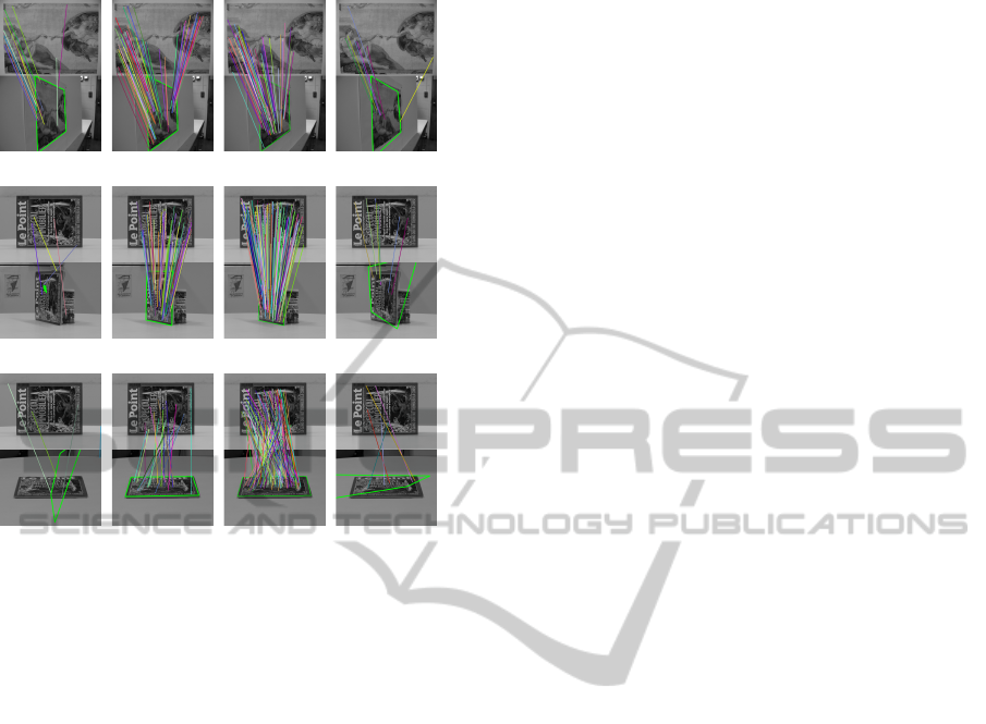
ASIFT can get most points of correspondence but

its precision is not best in this experiment. In terms of

processing time, ASIFT takes 47 seconds per image

but SIFT VGL takes 3 seconds about Grafﬁti. There-

fore, ASIFT is not suitable for fast run-time purpose,

while VGL can ensure the faster computation with

higher accuracy.

On the other hand, Ferns generally performs much

faster than local features matching method but it is not

very robust to camera movements. Its learning also

takes a long time due to huge patch training; more

than 10 minutes about Grafﬁti. In contrast, VGL per-

forms highly accurately with short learning time (less

than 15 seconds). Thanks to many widely spread cor-

respondences of stable keypoints, VGL can also cor-

rectly estimate a target pose even in the case of a large

viewpoint change. Meanwhile local features applying

VGL work until 80

◦

angle changes with fast learning,

less than quarter of a minute.

VISAPP2013-InternationalConferenceonComputerVisionTheoryandApplications

314

Default SIFT VGL for SIFT ASIFT Ferns

14/33 (42%) 83/111 (75%) 80/149 (54%) 7/10 (70%)

0/51 (0%) 81/128 (63%) 245/437 (56%) 8/16 (50%)

0/12 (0%) 24/37 (65%) 125/235 (53%) 2/10 (20%)

Figure 6: The keypoints of correspondence and the pose

estimation result in Adam and Magazine. These numbers

show the correct matches / all matches.

6 CONCLUSIONS

We have presented a stable keypoint recognition that

is robust to viewpoint changes. By generating var-

ious patterns as seen from different viewpoints and

the clusterization of the collected local invariant fea-

tures, our system learns a set of descriptors under var-

ious camera poses for each keypoints before actual

matching. This learning achieves more repeatability

and precision while maximizing each local feature’s

inherent advantage, and takes less than quarter of a

minute.

Recent years the evaluation research for the com-

bination of local feature detector and descriptor have

been done (Gauglitz et al., 2011). As any local fea-

ture descriptor algorithm that is described as a high

dimensional value can be applied to our framework,

in the case of feature with low scale or rotation invari-

ance, we can still apply our method after generating a

new viewpoint pattern to cover that situation.

REFERENCES

Agrawal, M., Konolige, K., and Blas, M. R. (2008). Cen-

sure: Center surround extremas for realtime feature

detection and matching. ECCV, 5305:102–115.

Arthur, D. and Vassilvitskii, S. (2007). k-means++: The ad-

vantages of careful seeding. Proceedings of the eigh-

teenth annual ACM-SIAM symposium on Discrete al-

gorithms, pages 1027–1035.

Baumberg, A. (2000). Reliable feature matching across

widely separated views. CVPR, pages 774–781.

Bay, H., Tuytelaars, T., Gool, V., and L. (2006). Surf:

Speeded up robust features. ECCV, 3951:404–417.

Bellavia, F., Tegolo, D., and Trucco, E. (2010). Improv-

ing sift-based descriptors stability to rotations. ICPR,

pages 3460–3463.

Brown, M. and Lowe, D. (2002). Invariant features from

interest point groups. BMVC, pages 656–665.

Gauglitz, S., Hollerer, T., and Turk, M. (2011). Evaluation

of interest point detectors and feature descriptors for

visual tracking. IJCV, 94:335–360.

Lepetit, V. and Fua, P. (2006). Keypoint recognition us-

ing randomized trees. IEEE Transactions on Pattern

Analysis and Machine Intelligence, 28(9):1465–1479.

Lieberknecht, S., Benhimane, S., Meier, P., and Navab, N.

(2009). A dataset and evaluation methodology for

template-based tracking algorithms. ISMAR, pages

145–151.

Lowe, D. G. (2004). Distinctive image features from scale-

invariant keypoints. IJCV, 60:91–110.

Mikolajczyk, K. and Schmid, C. (2004). Scale & afﬁne

invariant interest point detectors. IJCV, 60:63–86.

Mikolajczyk, K. and Schmid, C. (2005). A performance

evaluation of local descriptors. IEEE Transactions on

Pattern Analysis and Machine Intelligence, 27:1615–

1630.

Mikolajczyk, K., Tuytelaars, T., Schmid, C., Zisserman, A.,

Matas, J., Schaffalitzky, F., Kadir, T., and Van Gool,

L. (2005). A comparison of afﬁne region detectors.

IJCV, 65:43–72.

Morel, J. M. and Yu, G. (2009). Asift: A new framework for

fully afﬁne invariant image comparison. SIAM Jour-

nal on Imaging Sciences, 2(2):438–469.

Ozuysal, M., Calonder, M., Lepetit, V., and Fua, P. (2009).

Fast keypoint recognition using random ferns. IEEE

Transactions on Pattern Analysis and Machine Intel-

ligence, 32(3):448–461.

Takacs, G., Chandrasekhar, V., Chen, H., Chen, D., Tsai,

S., Grzeszczuk, R., and Girod, B. (2010). Permutable

descriptors for orientation-invariant image matching.

SPIE.

StableKeypointRecognitionusingViewpointGenerativeLearning

315