Finger Joint Characterization from X-Ray Images for Rheumatoid

Arthritis Assessment

Joan M. N´u˜nez, D´ebora Gil and Fernando Vilari˜no

Dept. of Comp. Science, Comp. Vision Center, Ediﬁci O - UAB, 08193 Bellaterra, Spain

Keywords:

Rheumatoid Arthritis, X-Ray, Hand Joint, Sclerosis, Sharp Van der Heijde.

Abstract:

In this study we propose a modular system for automatic rheumatoid arthritis assessment which provides a joint

space width measure. A hand joint model is proposed based on the accurate analysis of a X-ray ﬁnger joint

image sample set. This model shows that the sclerosis and the lower bone are the main necessary features in

order to perform a proper ﬁnger joint characterization. We propose sclerosis and lower bone detection methods

as well as the experimental setup necessary for its performance assessment. Our characterization is used to

propose and compute a joint space width score which is shown to be related to the different degrees of arthritis.

This assertion is veriﬁed by comparing our proposed score with Sharp Van der Heijde score, conﬁrming that

the lower our score is the more advanced is the patient affection.

1 INTRODUCTION

Rheumatoid arthritis (RA) is a chronic disease that

causes joint dysfunction which results, among other

symptoms, in the reduction of the joint space width

(JSW) and the erosion of the joint bones. Since there

is not any cure for RA, the assessment of the disease

becomes very important and it has led to the emer-

gence of several semi-quantitative assessment meth-

ods. Among them, the Sharp-Van der Heijde (SvdH)

score, which provides separate discrete values for

JSW and bone erosion based on X-ray image exam-

ination, is the most widely used nowadays (Van der

Heijde, 1999). The patient score is the sum of the

scores for all the considered joints in hands and feet.

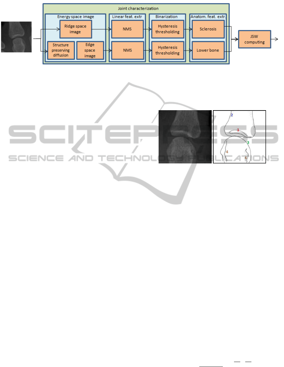
Three stages should be considered to face the au-

tomation of RA assessment: joint detection, joint

characterization and joint measurements. As the main

goal of this study is to propose and assess a JSW mea-

sure we will focus on the second and third stages tak-

ing hand joints as input (Figure 1). This statement

leads us to a hand joint modelling to describe the nec-

essary features to compute JSW measures. Sclerosis

and lower bone appear to be the main necessary fea-

tures to obtain JSW measures and the corresponding

detectors are proposed.

Few previous works have faced this problem. Bi-

elecki et al. (Bielecki et al., 2008) developed the ﬁrst

study that faced the challenge of a fully automatic sys-

tem for RA assessment. Vera et al. (Vera, 2010) pro-

vided a method which included all the different stages

of the problem improving signiﬁcantly the joint de-

tection rates. Langs et al. (Langs et al., 2009) pre-

sented a new method whose scope is also the whole

RA assessment process. However, these works faced

the problem as a whole stage, not modular, and did

not show a clear correlation among its proposed JSW

score and Svdh.

Our proposal clearly separates joint detection,

joint characterization and joint measurements in three

independent modules. It also provides a framework

for sclerosis and lower bone detection performance

assessment, and proposes a JSW score which exhibits

a close relation with SvdH score. This approach al-

lows us to conﬁrm for the ﬁrst time a relation between

an automatic score and the RA disease stage. More-

over, the modular orientation of our contribution, un-

like previous approaches, enables future research to

speciﬁcally focus on the improvement of the different

open challenges independently.

2 DATA ANALYSIS

This study is focused on the same digital database

used by Vera et al. (Vera, 2010) enriched with our

own manually segmented ground truth for the se-

lected visual features necessary for JSW computation.

Twenty X-ray images from different patients contain-

ing pairs of hands in posterioanterior view are avail-

288

Núñez J., Gil D. and Vilariño F..

Finger Joint Characterization from X-Ray Images for Rheumatoid Arthritis Assessment.

DOI: 10.5220/0004327302880292

In Proceedings of the International Conference on Biomedical Electronics and Devices (BIODEVICES-2013), pages 288-292

ISBN: 978-989-8565-34-1

 2013 SCITEPRESS (Science and Technology Publications, Lda.)

Figure 1: Rheumatoid Arthritis characterization system.

able in DICOM format, 2828x2320 resolution and in-

tensity range from 0 to 4095. Hand joints have been

marked by an expert who was asked to spot the joint

middle point along the ﬁnger axis and the joint ori-

entation. A hand joint dataset containing 560 images

of joints have been created (14 joints/hand). Among

these samples, a total number of 320 joints were

labelled with their SvdH score for inter-phalangeal

distance (discrete values from 0 to 3). These 320

samples comprised 160 metacarpo-phalangeal joints

(MCP) and 160 proximal inter-phalangeal joints (PIP)

-distal inter-phalangeal joints (DIP) are not consid-

ered within SvdH score-. Erosion scoring was not col-

lected because it is out of the scope of this this study.

Our proposed hand joint model does not consider

thumb joints as they represent a different problem due

to its speciﬁc proﬁle. Since images are taken with the

hands in posterioanterior view -from the hand back

with the palm facing down- a proﬁle view of the

thumb is taken. Consequently, a frontal projection

is obtained for the rest of the ﬁngers whereas a lat-

eral projection is obtained for the thumbs. This rea-

son, as well as their speciﬁc skeletal structure, causes

the visual features observed in thumbs to be substan-

tially different and justiﬁes that they are not included

in this study. As far as the other ﬁnger joints are

concerned, several features are distinguished within

the model: sclerosis, upper bone contour, lower bone

contour and lower bone inner edges, as depicted in

Figure 2 (N´u˜nez et al., 2011). The sclerosis and the

lower bone contour are the main necessary features to

carry out measures on JSW. The sclerosis (feature 1

in Figure 2(b)) appears as a consequence of the up-

per bone shape and the way an X-ray image is cre-

ated. The X-ray beam have to pass through a higher

density region due to the concavity of the lower part

of the upper bone of the joint (feature 2 in Figure

2(b)). As a consequence, the sclerosis appears as a

prominent high intensity region. Regarding the lower

bone, the visual features are also a consequence of the

mentioned X-ray image acquisition mechanism and

the lower bone shape (feature 3 in Figure 2(b)). That

shape can vary in the different ﬁngers or the different

hand joints and the inner edges may be present or not

(feature 4 in Figure 2(b)). However, the lower bone

contour is deﬁned by the outer part of the lower bone.

(a) (b)

Figure 2: (a) Joint example. (b) Joint model schema (1:

sclerosis, 2: upper bone, 3: lower bone, 4: inner edges).

3 METHODOLOGY

Our proposed sclerosis and lower bone detectors in-

clude several stages: energy space image, linear fea-

ture extraction, binarization and anatomical feature

extraction.

The ﬁrst stage aims to obtain the energy space im-

age. The intensity levels of that image describe the

chances of ﬁnding a feature in every pixel. Two sepa-

rate processes are achieved in order to obtain the ridge

space image and the edge space image. A second

derivative of anisotropic Gaussian (DoG) method is

used to compute the ridge space image. This method

is based on the fact that ridges can be obtained as

the high values in the second derivative. We apply a

bank of ﬁlters where each of them achieves a convo-

lution with the corresponding kernel template. We de-

sign our ﬁlter templates based on second derivatives

of anisotropic Gaussian kernels. Considering that an

oriented Gaussian function is described by:

(σ

,σ

),θ

(2π)σ

−



˜x

2σ

˜y

2σ



(1)

where (σ

, σ

) are the scales in the corresponding

axis, θ is the rotation angle of the ﬁlter and ˜x and ˜y

FingerJointCharacterizationfromX-RayImagesforRheumatoidArthritisAssessment

289

are the coordinates given by the rotation angle. Hence

they are deﬁned as:

˜x = xcosθ+ ysinθ

˜y = xsinθ − ycosθ

(2)

We use anisotropic Gaussians with σ = σ

= 2σ

Therefore, the Gaussian function results in:

σ,θ

(2π)2σ

−



˜x

2(2σ)

˜y

2σ



(3)

Hence the kernel will be deﬁned as:

∂

˜y

σ,θ

˜y

− 1

σ,θ

(4)

We apply a normalization so that the geometry of

the valleys is prioritized:

σ,θ

k∂

˜y

σ,θ

∗ Ik

k∂

˜y

σ,θ

kkIk

(5)

where k · k stands for the L

integral norm and ∗ de-

noting the convolution operator.

The kernels are applied to different scales and in

different equally distributed orientations in a range

centered in the joint orientation. The ﬁnal outcome

are 24 output images, each of them corresponding to

a determined orientation and scale. Hence, the output

ridges

must be a combination of all of them, deﬁned

as the maximum of the outputs from each ﬁlter:

ridges

= max

i, j



,θ



(6)

On the other hand, the edge space image is ob-

tained as the gradient of the input image after apply-

ing structure preserving diffusion (Gil et al., 2009).

Diffusion ﬁltering proved its success in improving the

quality of the edge detection by smoothing the image

irregularities while keeping the main image structure.

The second stage performs the feature extraction

using Non-maximum Suppresion algorithm (Canny,

1986), which only keeps pixels that are local maxima

along the gradient direction. Gradients are computed

using the structure tensor of the space image.

In the third stage hysteresis thresholding algo-

rithm (Canny, 1986) is used to binarize the non-

maximum suppressed images while preserving fea-

ture connectivity and removing weak responses.

Finally, the two images forwarded by the third

stage must go through the fourth processing step in or-

der to provide the ﬁnal sclerosis and lower bone seg-

mentations. This stage is different for the two thresh-

olded images:

• The ﬁnal sclerosis segmentation is the ridge in the

binarized image that is closer to the center of the

image following the ﬁnger orientation .

• As far as lower bone is concerned, the correspond-

ing binarized image is processed to remove the

edges in the upper part and the margins. After-

wards, the endpoints in the remaining processed

edges are linked. The ﬁnal lower bone segmenta-

tion is obtained by computing the convex hull of

the linked-edge image.

4 EXPERIMENTAL SETUP

Two subsets were created from our dataset of 320 an-

notated images to perform our experiments: 1) Tune

Dataset, with 40 randomly selected healthy joints (20

MCP and 20 PIP); 2) Test Dataset, with the remaining

280 joints (140 MCP and 140 PIP). The Tune Dataset

was used to tune the parameters of the system for scle-

rosis and lower bone contour segmentation, and the

Test Dataset was used to compute the output of our

system and compare the proposed distance measure

with the SvdH score. We added 20 DIP joints from

the non-annotated dataset to enrich the variability of

the Tune Dataset -these joints can be safely included

because, although not having a SvdH score, they ﬁt

our model-. Both sclerosis and lower bone were man-

ually segmented by an expert using OsiriX (Rosset

et al., 2004) software exclusively for the 60 images of

the Tune Dataset.

Performance metrics were developed to evaluate

the performance of the system, i.e. the quality of our

detections, and tune the parameters. We based our

metrics on the Average Surface Distance (ASD), de-

ﬁned as follows:

ASD(U, V) =

|S(U)|

∑

∈S(U)

d(s

, S(V))

(7)

where, given a pixel p and a region R conformed by a

set of pixels S(R), d(p, S(R)) is deﬁned as:

d(p, S(R)) = min

∈S(R)

kp − S

k (8)

where k.k stands for the Euclidean distance.

Thus, if A denotes our automatic segmentation and

M denotes the manual delineation, we deﬁne:

Caught = ASD(A, M) (9)

Missed = ASD(M, A) (10)

When both Caught and Missed metrics are zero

the segmentation is perfect. Caught metric value is

related to the quality of the detector at detecting valid

pixels (true positives) and avoiding non-desired pix-

els (false positives). Analogously, the lower the value

of Missed, the less desired information was missed

(false negatives).

BIODEVICES2013-InternationalConferenceonBiomedicalElectronicsandDevices

290

Table 1: Valid sclerosis and lower bone detection rates.

J. type SvdH 0 SvdH 1 SvdH 2 SvdH 3 Total

Sclerosis

MCP 111/115 (96.5%) 10/11 (90.9%) 10/12 (83.3%) 2/2 (100.0%) 133/140 (95.0%)

PIP 64/67 (95.5%) 27/35 (77.1%) 22/28 (78.5%) 5/10 (50.0%) 118/140 (84.2%)

Total 175/182 (96.1%) 37/46 (80.4%) 32/40 (80.0%) 7/12 (58.3%) 251/280 (89.4%)

L. bone

MCP 85/115 (73.9%) 5/11 (45.4%) 8/12 (66.6%) 0/2 (0.0%) 98/140 (70.0%)

PIP 42/67 (62.6%) 14/35 (40.0%) 8/28 (28.5%) 3/10 (30.0%) 67/140 (47.8%)

Total 127/182 (69.7%) 19/46 (41.3%) 16/40 (40.0%) 3/12 (25.0%) 165/280 (58.9%)

Table 2: Valid sclerosis and lower bone detection rates (both in the same image).

J. type SvdH 0 SvdH 1 SvdH 2 SvdH 3 Total

MCP 83/115 (72.1%) 5/11 (45.4%) 6/12 (50.0%) 0/2 (0.0%) 94/140 (67.1%)

PIP 39/67 (58.2%) 11/35 (31.4%) 6/28 (21.4%) 2/10 (20.0%) 58/140 (41.4%)

Total 122/182 (67.0%) 16/46 (34.7%) 12/40 (30.0%) 2/12 (16.6%) 152/280 (54.2%)

This experimental setup was used in order to train

the detection systems with the Tune Dataset. The

system providing the lowest values for the perfor-

mance metrics was selected, giving priority to a lower

Caught value so that the provided output is better al-

though some parts may be missed. Afterwards, the

selected detectors were applied to the Test Dataset.

The ﬁnal sclerosis and lower bone outputs were then

visually tested in order to separate the wrong detec-

tions from those detections that can be useful to com-

pute JSW scores. The ﬁnal detections were accepted

if they provided a good segmentation and there were

not remaining spurs in the joint interspace.

Finally, the proposed JSW measurement is the

minimum distance between the sclerosis and the

lower bone. It is deﬁned as:

min

= min

p∈L

d(p, S) (11)

where S and L stand for the sclerosis surface and the

lower bone contour, respectively.

5 RESULTS

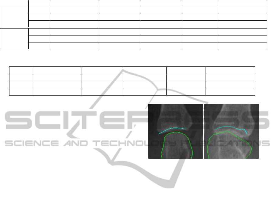
Table 1 shows the valid sclerosis and lower bone

rates when applying our sclerosis detector to the Test

Dataset. High detection rates have been obtained in

the case of sclerosis detection, reaching higher rates

in the case of healthy samples (SvdH 0), providing

96.1%, since they are closer to our joint model. How-

ever, these detection rates drop down to 58.3% in the

case of joints in a more advanced RA stage, which

makes clear the potential usefulness of the model in

order to classify advanced stages of the disease. All

in all, the detection rate reaches the remarkable value

of 89.6% on the whole dataset. As far as MCP and

PIP are concerned, the detection rates remain close

(a) (b)

Figure 3: (a) MCP valid detection. (b) MCP wrong detec-

tion.

although a light tendency is conﬁrmed which shows

that PIP joints present more detection problems.

On the other hand, lower bone detection arises as

a very difﬁcult problem. The overall detection rate

drops to 58.9% although the healthy samples reach

69.7%. The lack of an stardard practice in X-ray im-

age techniques causes an important variability in the

samples which makes lower bone segmentation difﬁ-

cult to achieve. Figure 3 shows two detection exam-

ples of wrong and valid segmentations.

The samples where both lower bone and sclerosis

segmentations were labelled as valid were considered

for further analysis. Table 2 contains the correspond-

ing results. The rates when the two segmentations are

considered altogether are just slightly below the lower

bone detection rates, reaching 67.0% for healthy sam-

ples and 54.2% for the whole dataset.

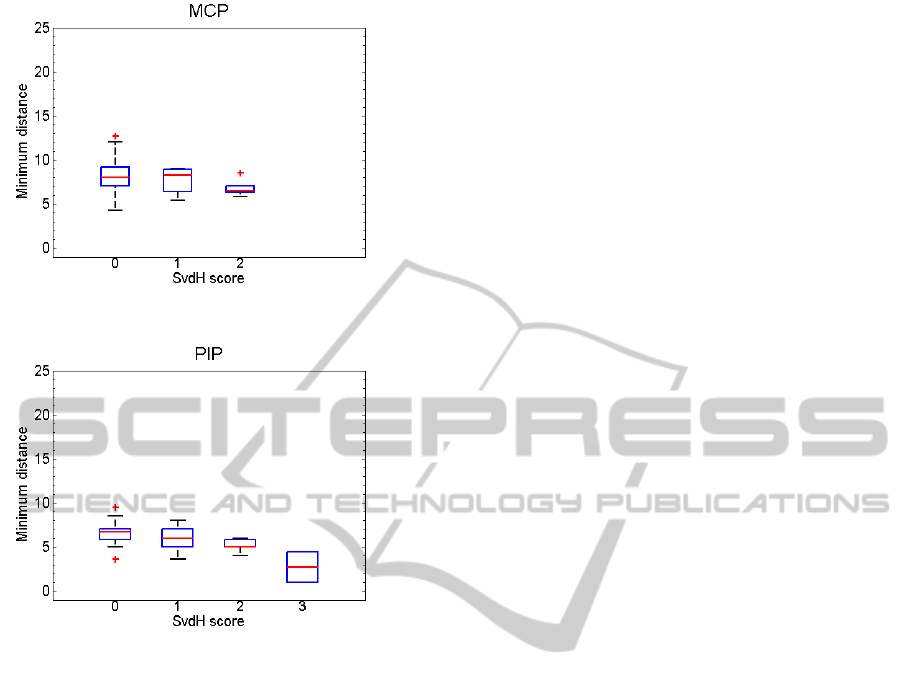
Afterwards, the proposed JSW measure was com-

puted and tested in relation to SvdH score. In the

case of MCP samples (Figure 4), the JSW estimation

shows a light decreasing trend as the value of SvdH

score increases. Nevertheless, that decreasing trend

is clear in the case of PIP samples (Figure 5). It is an

encouraging result taking into account that our system

is only considering JSW values. Standard clinical as-

sessment considers more information as the symme-

FingerJointCharacterizationfromX-RayImagesforRheumatoidArthritisAssessment

291

Figure 4: MCP joints, distance measure and SvdH score.

Figure 5: PIP joints, distance measure and SvdH score.

try between hand joints or erosion information.

Finally, the reliability of the proposed system to

provide a proper JSW estimation independently of its

relation to the RA stage was tested. The JSW measure

was computed both for the manual and automatic seg-

mentations of the Tune Dataset, providing a ﬁnal error

of 1± 0.7 pixels. This result conﬁrms the robustness

of the JSW estimation.

6 CONCLUSIONS

The proposed system sets the foundations of a mod-

ularized RA assessment system. We created a hand

joint sample dataset and introduced a hand joint

model based on the skeletal structure of hand bones.

Our sclerosis detector achieves remarkably good re-

sults. However, lower bone segmentation appears to

be a harder task when faced in a local way. The

JSW measure we propose was compared with the gold

standard score for RA assessment. We showed for the

ﬁrst time that an automatic measure for JSW can be

computed so that its value has a clear relation to the

SvdH manual measure assessed by clinical person-

nel and, therefore, to RA disease stage. Future work

should involve the conﬁrmation of this trend with a

dataset which should include a larger study with sam-

ples from multiple sources. Higher SvdH score sam-

ples, particularly scarce in number should be also con-

sidered.

ACKNOWLEDGEMENTS

This work was supported in part by the Spanish Gov.

grants TIN2012-33116, TIN2009-13618, MICINN

TIN2009-10435 and Consolider 2010 MIPRCV

(CSD2007-00018), and the UAB grant 471-01-

2/2010. The second author has been supported by the

Ramon y Cajal Program.

REFERENCES

Bielecki, A., Korkosz, M., and Zielinski, B. (2008). Hand

radiographs preprocessing, image representation in

the ﬁnger regions and joint space width measurements

for image interpretation. PRn, 41(12):3786–3798.

Canny, J. (1986). A computational approach to edge detec-

tion. PAMI, (6):679–698.

Gil, D., Hern`andez-Sabat´e, A., Burnat, M., Jansen, S.,

and Mart´ınez-Villalta, J. (2009). Structure-preserving

smoothing of biomedical images. In Computer Anal-

ysis of Images and Patterns, pages 427–434. Springer.

Langs, G., Peloschek, P., Bischof, H., and Kainberger, F.

(2009). Automatic quantiﬁcation of joint space nar-

rowing and erosions in rheumatoid arthritis. Medical

Imaging, IEEE Transactions on, 28(1):151–164.

N´u˜nez, J., F., V., and D., G. (2011). Computer vision tech-

niques for characterization of ﬁnger joints in x-ray im-

ages. Technical report, Centre de Visi´o per Computa-

dor.

Rosset, A., Spadola, L., and Ratib, O. (2004). Osirix: An

open-source software for navigating in multidimen-

sional dicom images. Journal of Digital Imaging,

17:205–216. 10.1007/s10278-004-1014-6.

Van der Heijde, D. (1999). How to read radiographs accord-

ing to the sharp/van der heijde radiological assessment

in rheumatoid arthritis in long term studies. Journal

of Rheumatology, (26):743–745.

Vera, S. (2010). Finger joint modelling from hand x-ray

images for assessing rheumatoid arthritis. Technical

report, Centre de Visi´o per Computador.

BIODEVICES2013-InternationalConferenceonBiomedicalElectronicsandDevices

292