
The Impact the Price Promotion Has on the Manufacturer’s
Performance
Wenting Pan
1
, Yung-Jae
2
and Tina Zhang
3
1
School of Economics and Business Administration, Saint Mary’s College of California,
380 Moraga Road, 94556 Moraga, U.S.A.
2
Operations Management, Saint Mary’s College of California, 380 Moraga Road, 94556 Moraga, U.S.A.
3
Saint Mary’s College of California, 380 Moraga Road, 94556 Moraga, U.S.A.
Keywords: Price Promotion, Supply Chain, EOQ, EPQ.
Abstract: We consider a supply chain network where there is one manufacturer and multiple identical retailers in a
consumer non-durable market. The retail purchase price is exogenous, and demand is deterministic. The
retailers apply the Economic Order Quantity (EOQ) model to minimize the total cost. In observation of the
manufacturer’s periodic instantaneous promotion, the retailers would place a one-time order from the
manufacturer to take advantage of the deal during the promotion period. The objective of this paper is to
examine the impact this price promotion has on the manufacturer’s performance. We find that this
promotion policy has a negative impact on the manufacturer’s performance. Interestingly, we also find that
this negative impact is less damaging when the utilization of the facility is lower.
1 INTRODUCTION
Trade promotions are deep-rooted marketing
practices to temporarily increase sales volume,
especially in the consumer non-durable market. Even
though trade promotions are designed to serve
certain marketing objectives, they also create
inefficiency in distribution channels. Research
papers include Jones (1990), Buzzell et al., (1990)
and Ailawadi et al., (1999).
The purpose of this paper is to provide an
analytical framework to quantify the economic
impact the price promotions have on the
manufacturer’s performance.
2 THE BASIC FRAMEWORK
We consider a supply chain network, comprised of
one manufacturer and multiple identical retailers.
The retailer model studies the retailers’ purchasing
pattern and the manufacturer model focuses on the
optimal production schedule. Based on the results
derived from these two models, we can then analyze
the impact of price promotions on the
manufacturer’s performance.
The Retailer Model. Here are the assumptions for
the retailer model. Lead time is zero. Shortages are
not allowed. All the retailers are identical. The
manufacturer’s promotion period is instantaneous.
We further assume that the discount is offered by the
manufacturer at the beginning of each period. We
use the following notations throughout the paper for
the retailers:
D = the retailer’s demand per period (say, year)
assumed constant and uniform;
= retailer’s setup cost per order;
= retailer’s unit purchasing cost;
= retailer’s unit inventory holding cost per period,
expressed as a percentage of the value of the item;
= retailer’s order quantity
d = discount expressed as a percentage of price
during the promotion period.
Let
∗
denote the retailer’s optimal order quantity.
It is straightforward to see that when d = 0,
∗
is
solved by,
∗
.
(1)
We next consider the general case when 0.
Since the manufacturer offers a discount for a very
195
Pan W., Lee Y. and Zhang T..
The Impact the Price Promotion Has on the Manufacturer’s Performance.
DOI: 10.5220/0004341103430346
In Proceedings of the 2nd International Conference on Operations Research and Enterprise Systems (ICORES-2013), pages 343-346
ISBN: 978-989-8565-40-2
Copyright
c
2013 SCITEPRESS (Science and Technology Publications, Lda.)

short period of time, the retailer only makes a one-
time purchase during the promotion period to take
advantage of the discount. After the short promotion
time, the retailer resumes its economic order
quantity
∗
for the rest of this period until the next
discount occurs at the beginning of the next period.
In particular, let
be this one time order quantity.
Since we assume that the discounts are offered by
the manufacturer regularly, the retailer has no reason
to order more than units when the deal is on. Thus,
we can restrict
without loss of generality. It
follows that the retailer’s total cost in one period is
given by
=
1
1
∗
1
∗
1
.
(2)
Differentiating
with respect to
, we
obtain
2
1
(3)
and
1
0.
(4)
Hence,
is convex in
and the optimal
order quantity, denoted by
∗
,is uniquely solved by
equation
0. It directly follows that
∗
1
2
1
.
(5)
Clearly that
∗
is strictly increasing in the discount
level d. Furthermore, notice that
∗
∗
when
0. Thus,
∗
∗
. Since the retailer would
never order more than units when the deal is on,
the maximum level of discount
̅
is given by
= 1,
(6)
or equivalently
̅
1
.
(7)
Clearly, for any
̅
, the retailer would order
units at the discount price. Therefore, we shall
assume that
̅
in the following analysis, and
so
∗
.
Let α denote the proportion of the one-time
purchase out of its total demand when the price
discount is offered, i.e.,
α =
∗
1.
(8)
2.1 The Manufacturer Model
The manufacturer model studies the optimal
production schedule that minimizes the
manufacturer’s production and inventory holding
costs given the retailers’ purchasing pattern and the
capacity of the manufacturer’s facility. In this model,
we assume that there are many identical individual
retailers who independently make purchasing
decisions from this manufacturer. Here are the
notations we will use throughout the paper for the
manufacturer.
= the manufacturer’s setup cost per order;
= the manufacturer’s unit production cost;
= the manufacturer’s unit holding cost per period,
expressed as a percentage of the value of the item;
μ = the manufacturer’s production rate per period;
λ = the manufacturer’s aggregate demand rate per
period.
ρ =
, utilization of the manufacturer’s facility.
The retailer model discussed in Section 2.1 suggests
that individual retailer purchases a certain portion
(α) of its total one-period demand when the discount
is offered at the beginning of each period. Since we
assume identical retailers, it is clear that α portion of
the aggregate demand λ occurs when the discount is
offered at the beginning of the period, with no
demand for the following α period of time, and the
remaining demand (λ - αλ) occurs for the next
(1 – α) period of time. We assume that demand (λ -
αλ) occurs uniformly between time (1 – α) and time
1.
We now study the manufacturer’s optimal
production schedule that minimizes the total cost.
There exist four cases depending on the value of α
and the utilization of the facility ρ.
Case (i) 01 and 1
Case (i) represents the situation where some discount
is offered at the beginning of each period and the
utilization of the facility is lower than a
threshold1. In this case, the manufacturer
would start to build up the inventory at time [1-
–
so that he can get ready for the price
promotion that occurs at the beginning of the next
time period. Therefore, the last production run in this
period begins at time [1-
–
.
We next adopt the idea of the Economic
ICORES2013-InternationalConferenceonOperationsResearchandEnterpriseSystems
196

Production Lot Size model to approximate the
manufacturer’s optimal production quantity. We
shall determine the optimal number of production
runs between the time period and time period (1-
–
). Let n denote the number of production runs
between the time period and time period (1-
–
).
The production and inventory costs are given by
=
+
1
(9)
To simplify the analysis, we here assume that is a
real number. Clearly, the optimal number of the
production runs, denoted by
∗
, is given by
∗
=
.
(10)
It directly follows that the optimal manufacturer’s
cost
∗
2
2
21
.
(11)
Case (ii) 01 and 1
Case (ii) represents the situation where some
discount is offered at the beginning of the period and
the utilization of the facility is higher than the
threshold
1
.
During the first α period of time when there is no
demand, the manufacturer’s inventory level can be
increased with the rate of μ if there is a production
run. The manufacturer’s inventory level can be
accumulated with the rate of (μ – λ) during the
remaining (1 – α) period of time when the demand
occurs at the rat of λ. Therefore, to accumulate αλ
units at the end of the period, the manufacturer must
start the production run at time (1 – ρ).
Thus, the production and inventory costs are given
by
+
+
.
(12)
Case (iii) 01 and 1
In this case, the facility is dedicated to making just
one specific product without any excess capacity.
During the first α period of time when there is no
demand, the manufacturer would build up αλ units of
the product to meet the demand at the beginning of
the next period. The manufacturer would then hold
this amount of inventory for the remaining (1 – α)
period of time since the demand rate λ is equal to the
production rate μ.
Thus, the production and inventory costs are
given by
1
.
(13)
Case (iv) α = 1 and ρ < 1
This case corresponds to the situation where
̅
.
Since the discount is so large, the retailers purchase
the entire one-period demand when the discount is
offered. In this case, the manufacturer must start
building up the entire amount of one period demand
λ at time (1 – ρ). The entire amount would be sold to
the retailers at the beginning of the next period.
Thus, the production and inventory costs are
given by
.
(14)
2.2 Model Combination
Clearly, the manufacturer’s revenue is equal to αλ (1
– d)
+ (1 - λ
. Let
denote the profit for case i.
= αλ (1 – d)
+ (1 - λ
2
.
(15)
= αλ (1 – d)
+ (1 – λ
+
+
.
(16)
= αλ (1 – d)
+ (1 – λ
[
1
.
(17)
= αλ (1 – d)
+ (1 – λ
.
(18)
3 NUMERICAL EXAMPLES
We have conducted extensive numeral experiments
to understand the impact this price promotion has on
the manufacturer’s performance.
Consider the following parameters for the
retailers: D = 10,000,
= 70,
= 0.4, and
= 200;
and the following parameters for the manufacturer: μ
= 100,000,
= 50,
0.3, and
1,000.
Three levels of aggregate demand are: λ = 50,000, λ
= 70,000, λ = 90,000. Therefore, the corresponding
TheImpactthePricePromotionHasontheManufacturer'sPerformance
197
utilization is 0.5, 0.7, and 0.9 respectively.
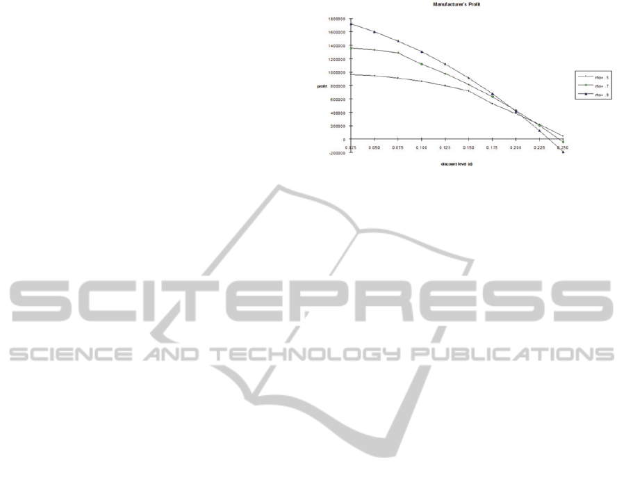
Observation: The Manufacturer’s Profit
Decreases as the Level of Discount Increases.
Furthermore, the Marginal Decrease is Higher
when the Utilization of the Facility is Higher.
Figure 1 illustrates the relationship between the
manufacturer’s profit and the level of discount
offered by the manufacturer. As shown in Figure 1,
the profit decreases as the discount level increases
for all three different levels of utilization. Figure 1
also shows that the marginal decrease is higher when
the utilization of the facility is higher, as the
discount level increases.
Interestingly, at 0.225 discount level , the
manufacturer’s profit when the utilization of the
facility is 0.5 is higher than the manufacturer’s profit
when the utilization of the facility is 0.7 and 0.9.
This implies that the detrimental effect of trade deals
on manufacturer’s profit is not so severe when the
manufacturer has a relatively large capacity cushion
or equivalently, the manufacturer operates at a low
rate. Even though the promotion deal helps decrease
the inventory level faster due to the larger order
quantities from the retailers, this benefit is usually
offset by the fact that the manufacturer has to
prepare for the deal. Since the manufacturer has to
start the production much earlier than he would
when there was no deal offered to the retailers, the
manufacturer has to carry extra inventory, which
increases the inventory holding cost. However, if the
manufacturer has large enough capacity, he does not
need to start the production too early, thus
decreasing the time to carry inventory before and
after the completion of a production run.
4 CONCLUSIONS
In this paper, we develop a framework to study the
impact the price promotion has on the
manufacturer’s performance, taking into account the
retailers’ purchasing pattern, under deterministic
demand. We find that the price promotion has a
negative impact on the manufacturer’s performance.
We also find that the detrimental effect of the price
promotion is less damaging when the facility
utilization is lower. Price sensitive demand is of
great interest for the further research, especially the
stochastic case. Different but interesting insights
might be derived if price promotions affect the total
aggregate demand.
Figure 1: Manufacturer’s profit versus discount level.
REFERENCES
Ailawadi K., P. Farris, and E. Shames, (1999): “Trade
Promotion: Essential to Selling through Resellers”,
Sloan Management Review, 41, 1, 83-96.
Buzzell, R. D., J. A. Quelch, and W. J. Salmon, (1990):
“The Costly Bargain of Trade Promotion”, Harvard
Business Review, 68, 2, 141-149.
Jones, J. P. (1990): “The Double Jeopardy of Sales
Promotions”, Harvard Business Review, 68, 5, 145-
152.
ICORES2013-InternationalConferenceonOperationsResearchandEnterpriseSystems
198
