Artificial Neural Network based Methodologies

for the Spatial and Temporal Estimation of Air Temperature

Application in the Greater Area of Chania, Greece

Despina Deligiorgi

, Kostas Philippopoulos

and Georgios Kouroupetroglou

Division of Environmental Physics and Meteorology, Department of Physics, University of Athens, Athens, Greece

Division of Signal Processing and Communication, Department of Informatics and Telecommunications,

University of Athens, Athens, Greece

Keywords: Air Temperature Prediction, Artificial Neural Networks, Time-series Forecasting, Spatial Interpolation.

Abstract: Artificial Neural Networks (ANN) propose an alternative promising methodological approach to the

problem of time series assessment as well as point spatial interpolation of irregularly and gridded data.

ANNs can be used as function approximators to estimate both the time and spatial air temperature

distributions based on observational data. After reviewing the theoretical background as well as the relative

advantages and limitations of ANN methodologies applicable to the field of air temperature time series and

spatial modelling, this work focuses on implementation issues and on evaluating the accuracy of the AAN

methodologies using a set of metrics in the case of a specific region with complex terrain. A number of

alternative feed forward ANN topologies have been applied in order to assess the spatial and time series air

temperature prediction capabilities in different horizons. For the temporal forecasting of air temperature

ANNs were trained using the Levenberg-Marquardt back propagation algorithm with the optimum

architecture being the one that minimizes the Mean Absolute Error on the validation set. For the spatial

estimation of air temperature the Radial Basis Function and Multilayer Perceptrons non-linear Feed Forward

AANs schemes are compared. The underlying air temperature temporal and spatial variability is found to be

modeled efficiently by the ANNs.

1 INTRODUCTION

Air temperature measurements in high resolution

time series are available only at limited stations

because meteorological data are generally recorded

at specific locations and derived from different

meteorological stations with non-identical

characteristics. Spatial interpolation approaches

essentially transfer available information in the form

of data from a number of adjacent irregular sites to

the estimated sites. Thus, spatial interpolation

methods are frequently used to estimate values of air

temperature data in locations where they are not

measured. Various methods have been developed

with the purpose to compare the performance of

different traditional spatial interpolation methods for

air temperature data (Price et al., 2000); (Chai et al.

2011). Accurate ambient temperature estimates are

important not only in spatial but also in temporal

scales. Air temperature time series forecasting is one

of the most significant aspects in environmental

research and in climate impact studies. Time series

forecasts are valuable in renewable energy industry,

in agriculture for estimating potential hazards, and

within an urban context, in air quality studies for

assessing the risk of adverse health effects in the

general population.

During the last few decades, there has been a

substantial increase in the interest on Artificial

Neural Networks (ANN). ANNs have been

successfully adopted in solving complex problems in

many fields. Essentially, ANNs provide a

methodological approach in solving various types of

nonlinear problems that are difficult to deal with

using traditional techniques. Often, a geophysical

phenomenon exhibits temporal and spatial

variability, and is suffering by issues of nonlinearity,

conflicting spatial and temporal scale and

uncertainty in parameter estimation (Deligiorgi and

Philippopoulos, 2011). ANNs have been proved

(Deligiorgi et al., 2012) to be flexible models that

669

Deligiorgi D., Philippopoulos K. and Kouroupetroglou G..

Artiﬁcial Neural Network based Methodologies for the Spatial and Temporal Estimation of Air Temperature - Application in the Greater Area of Chania,

Greece.

DOI: 10.5220/0004373906690678

In Proceedings of the 2nd International Conference on Pattern Recognition Applications and Methods (PRG-2013), pages 669-678

ISBN: 978-989-8565-41-9

 2013 SCITEPRESS (Science and Technology Publications, Lda.)

have the capability to learn the underlying

relationships between the inputs and outputs of a

process, without needing the explicit knowledge of

how these variables are related.

Recently, numerous applications of AANs to

estimate air temperature data have been presented,

e.g. in areas with sparse network of meteorological

stations (Snell et al., 2000); (Chronopoulos et al.,

2008) for the prediction of hourly (Tasadduq,

Rehman and Bubshait, 2002), daily (Dombayc and

Golcu, 2009) and year-round air temperature (Smith

et al., 2009) or room temperature (Mustafaraj et al.,

2011) as well as for simulating the Heat Island

(Mihalakakou et al., 2002).

In this work first we briefly present the

theoretical background of ANN methodologies

applicable to the field of air temperature time series

and spatial modeling. Next, we focus on

implementation issues and on evaluating the

accuracy of the aforementioned methodologies using

a set of metrics in the case of a specific region with

complex terrain at Chania, Crete Island, Greece. A

number of alternative Feed-forward ANN topologies

are applied in order to assess the spatial and time

series air temperature prediction capabilities in

different time horizons.

2 ANN PREDICTION MODELING

Artificial Neurons are Process Element (PE) that

attempt to simulate in a simplistic way the structure

and function of the real physical biological neurons.

A PE in its basic form can be modelled as non-liner

element that first sums its weighted inputs x

, x

...x

(coming either from original data, or from the

output of other neurons in a neural network) and

then passes the result through an activation function

Ψ (or transfer function) according to the formula:



















jjiii

wxy



(1)

where y

is the output of the artificial neuron, θ

is an

external threshold (or bias value) and w

are the

weight of the respective input x

which determines

the strength of the connection from the previous

PE’s to the corresponding input of the current PE.

Depending on the application, various non-linear or

linear activation functions Ψ have been introduced

(Fausett, 1994); (Bishop, 1995) like the: signum

function (or hard limiter), sigmoid limiter, quadratic

function, saturation limiter, absolute value function,

Gaussian and hyperbolic tangent functions. Artificial

Neural Networks (ANN) are signal or information

processing systems constituted by an assembly of a

large number of simple Processing Elements, as they

have been described above. The PE of a ANN are

interconnected by direct links called connections and

cooperate to perform a Parallel Distributed

Processing in order to solve a specific computational

task, such as pattern classification, function

approximation, clustering (or categorization),

prediction (or forecasting or estimation),

optimization and control. One the main strength of

ANNs is their capability to adapt themselves by

modifying the interaction between their PE. An-

other important feature of ANNs is their ability to

automatically learn from a given set of

representative examples.

The architectures of ANNs can be classified into

two main topologies: a) Feed-forward multilayer

networks (FFANN) in which feedback connections

are not allowed and b) Feedback recurrent networks

(FBANN) in which loops exist. FFANNs are

characterized mainly as static and memory-less

systems that usually produce a response to an input

quickly (Jain et al., 1996). Most FFANNs can be

trained using a wide variety of efficient conventional

numerical methods. FBANNs are dynamic systems.

In some of them, each time an input is presented, the

ANN must iterate for a potentially long time before

it produces a response. Usually, they are more

difficult to train FBANNs compared to FFANNs.

FFANNs have been found to be very effective

and powerful in prediction, forecasting or estimation

problems (Zhang et al., 1998). Multilayer

perceptrons (MLPs) and radial basis function (RBF)

topologies are the two most commonly-used types of

FFANNs. Essentially, their main difference is the

way in which the hidden PEs combine values

coming from preceding layers: MLPs use inner

products, while RBF constitutes a multidimentional

function which depends on the distance

cxr 

between the input vector x and the center c (where



denotes a vector norm) (Powell, 1987). As a

consequence, the training approaches between MLPs

and RBF based FFANN is not the same, although

most training methods for MLPs can also be applied

to RBF ANNs. In RBF FFANNs the connections of

the hidden layer are not weighted and the hidden

nodes are PEs with a RBF, however the output layer

performs simple weighted summation of its inputs,

like in the case of MLPs. One simple approach to

approximate a nonlinear function is to represent it as

a linear combination of a number of fixed nonlinear

ICPRAM2013-InternationalConferenceonPatternRecognitionApplicationsandMethods

670

RBFs



)(xz

, according to (2):









wxzx

)(

(2)

Typical choices for RBFs



cxFz



are:

piecewise linear approximations, Gaussian function,

cubic approximation, multiquadratic function and

thin plate splines.

A MLP FFANN can have more than one hidden

layer. But theoretical research has shown that a

single hidden layer is sufficient in that kind of

topologies to approximate any complex nonlinear

function (Cybenco, 1989); (Hornik et al., 1989).

There are two main learning approaches in

ANNs: i) supervised, in which the correct results are

known and they are provided to the network during

the training process, so that the weights of the PEs

are adjusted in order its output to much the target

values and ii) unsupervised, in which the ANN

performs a kind of data compression, looking for

correlation patterns between them and by applying

clustering approaches. Moreover, hybrid learning

(i.e. a combination of the supervised and supervised

methodologies) has been applied in ANNs.

Numerous learning algorithms have been introduced

for the above learning approaches (Jain et al., 1996).

The introduction of the back propagation

learning algorithm (Rumelhart et al., 1986) to obtain

the weight of a multilayer MLP could be regarded as

one of the most significant breakthroughs for

training AANs. The objective of the training is to

minimize the training mean square error E

mse

of the

AAN output compared to the required output for all

the training patterns:









kji

kmse

(3)

where: E

is the partial network error, p is the

number of the available patterns and Y the set of the

output PEs. The new configuration in time t > 0 is

calculated as follows:







jiji

kwkw



)1()(

(4)

)]2()1([  kwkw

jiji



To speed up the training process, the faster

Levenberg-Marquardt Back propagation Algorithm

has been introduced (Yu and Wilamowski, 2011). It

is fast and has stable convergence and it is suitable

for training AAN in small-and medium-sized

problems. The new configuration of the weights in

the k+1 step is calculated as follows:





)()()1(

kJIJJkwkw







(5)

The Jacobian matrix for a single PS can be written

as follows:



















www









(6)





















where: w is the vector of the weights, w

is the bias

of the PE and ε is the error vector, i.e. the difference

between the actual and the required value of the

ANN output for the individual pattern. The

parameter λ is modified based on the development of

the error function E.

3 APPLICATION OF ANN IN AIR

TEMPERATURE ESTIMATION

The present work aims to quantify the ability of

ANNs to estimate and model the temporal and

spatial air temperature variability at a coastal

environment. We focus on implementation issues

and on evaluating the accuracy of the

aforementioned methodologies in the case of a

specific region with complex terrain. A number of

alternative ANN topologies are applied in order to

assess the spatial and time series air temperature

prediction capabilities in different time scales.

Moreover, this work presents an attempt to

develop an extensive model performance evaluation

procedure for the estimation of the air temperature

using ANNs. This procedure incorporates a variety

of correlation and difference statistical measures. In

detail, the correlation coefficient (R), the coefficient

ArtificialNeuralNetworkbasedMethodologiesfortheSpatialandTemporalEstimationofAirTemperature-Application

intheGreaterAreaofChania,Greece

671

of determination (R

), the mean bias error (MBE),

the mean absolute error (MAE), the root mean

square error (RMSE) and the index of agreement (d)

are calculated for the examined predictive schemes.

The formulation and the applicability of such

measures are extensively reported in (Fox, 1981);

(Willmott, 1982).

3.1 Area of Study

The study area is the Chania plain, located on the

northwestern part of the island of Crete in Greece.

The greater area is constricted by physical

boundaries, which are the White Mountains on the

south, the Aegean coastline on the northern and

eastern part and the Akrotiri peninsula at the

northeast of Chania city (Figure 1). The topography

of the region is complex due to the geophysical

features of the region. The influence of the island of

Crete on the wind field, especially during summer

months and days where northerly etesian winds

prevail, is proven to cause a leftward deflection and

an upstream deceleration of the wind vector

(Koletsis, 2009); (Koletsis et al., 2010); (Kotroni,

2001). Moreover, the wind direction of the local

field at the broader area of Chania city varies

significantly due to the different topographical

features (Deligiorgi et al., 2007).

In this study, mean hourly air temperature data

are obtained from a network of six meteorological

stations, namely Airport, Souda, Platanias, Malaxa,

Pedio Volis and TEI (Figure 1). The measurement

sites cover the topographical and land-use variability

of the region (Table 1). The climatological station at

the Airport is representative of the meteorological

conditions that prevail at the Akrotiri peninsula and

in this application it will be used as the reference

station for examining the performance of the

temporal and spatial pattern recognition approaches.

TEI, Souda and Malaxa stations are situated along

the perpendicular to the Aegean coastline north-

south axis of the Chania basin,, while the TEI and

Platanias stations are representative of the coastal

character of the basin. Moreover, TEI station is

located at the east and in close proximity to the

densely populated urban district of Chania city.

The topography induces significant spatial air

temperature variation. In detail, the inland stations at

Souda and at the Airport exhibit the highest diurnal

temperature ranges (7.75 °C and 6.56 °C

respectively), while the spatial minimum is observed

at Pedio Volis (2.32 °C), a finding that is attributed

to the effect of altitude and the proximity of the site

to the Aegean coastline. The highest daily maximum

temperature values, averaged over the experimental

period, are reported at the Airport (24 °C) and the

lowest at Malaxa (19.46 °C).

3.2 Spatial Estimation of Air

Temperature

3.2.1 Implementation

For the spatial estimation of air temperature the non-

linear Feed Forward Artificial Neural Networks

MLPANN and RBFANN are compared. The method

aims to estimate air temperature at a target station,

using air temperature observations as inputs from

adjacent control stations.

The target station is located at Airport, while the

concurrent air temperature observations from the

remaining sites - control stations (Souda, Malaxa,

Platanias, PedioVolis and TEI) are used as inputs in

the MLPANN and RBFANN models.

The study period is from 19 July 2004 to 31

August 2006 and due to missing observations the

input datasets consist of 12416 simultaneous

samples of hourly observations for each station. The

60% of the available data (7450 cases from 19 July

2004 at 23:00:00 to 1 Oct. 2005 at 09:00:00) was

used for building and training the models (training

set), the subsequent 20% as the validation set (2483

cases from 1 Oct. 2005 at 10:00:00 to 26 March

2006 at 11:00:00) and the remaining 20% (2483

cases from 26 March 2006 at 12:00:00 to 31 Aug.

2006 at 22:00:00) as the test set which is used to

examine the performance of both the RBFANN and

the MLPANN models. In MLPANNs the validation

Table 1: Geographical characteristics of the meteorological stations.

Station Name Latitude (°N) Longitude (°W) Elevation (m) Characterization

Airport 24° 07΄ 00΄΄ 35° 33΄ 00΄΄ 140 Rural

TEI 35° 31΄ 09΄΄ 24° 02΄ 33΄΄ 38 Suburban – Coastal

Souda 35° 30΄ 30΄΄ 23° 54΄ 40΄΄ 118 Suburban

Platanias 35° 29΄ 46΄΄ 24° 03΄ 00΄΄ 23 Rural – Coastal

Malaxa 35° 27΄ 57΄΄ 24° 02΄ 33΄΄ 556 Rural

Pedio Volis 35° 34΄ 11΄΄ 24° 10΄ 20΄΄ 422 Rural

ICPRAM2013-InternationalConferenceonPatternRecognitionApplicationsandMethods

672

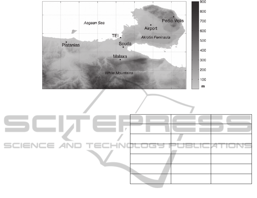
Figure 1: Area of study and location of meteorological stations.

set is used for early stopping and to determine the

optimum number of hidden layer neurons and in the

RBFANNs to determine the optimum value of the

spread parameter of the radial basis function. Large

spread values result into a smooth function

approximation that might not model the temperature

variability adequately, while small spread values can

lead to networks that might not generalize well. In

our case the validation set is used for selecting the

optimum value of the spread parameter, using the

trial and calculating the error procedure by

minimizing the MAE.

The optimum architecture for the MLPANN

model is 5-17-1 (5 inputs, 17 hidden layers and 1

output neuron). The RBFANN used had five inputs

and a radial basis hidden layer with 7450 artificial

neurons using Gaussian activation functions

radbas(n) = exp(-n

). The output layer had one PE

with linear activation function.

3.2.2 Results

The model evaluation statics for the Airport station

for both MLPANN and RBFANN approaches are

presented in Table 2. A general remark is that both

models give accurate air temperature estimates with

MAE values less than 0.9 °C and with very high d

values and minimal biases. Furthermore the

explained variance is 95.9% for the RBFANN model

and 96.3% for the MLPANN scheme. The metrics

indicate that MLPANN slightly outperforms the

trained RBFANN network.

The comparison of the observed and the

predicted air temperature values for both models are

presented in Figure 2 scatter plots and the respective

residuals’ distributions are given in Figure 3.

Limited data dispersion is observed for both models

and in both cases the residuals are symmetrically

distributed around 0 °C.

Table 2: ANN based model performance.

MLPANN RBFAAN

0.981

0.979

0.963

0.959

MBE (°C)

-0.008

0.034

MAE (°C)

0.819

0.871

RMSE (°C)

1.067

1.120

0.990

0.989

Moreover, a time series comparison between the

observed and the predicted air temperature form the

MLPANN and RBFANN models are presented in

Figure 4 for the period 10-23/8/2006. The predicted

air temperature time series follows closely the

observed values with no signs of systematic errors.

The temperature estimation errors are further

examined by calculating the MAE hourly values

(Figure 5). The analysis for both ANN models

reveals two maxima, which are observed during the

early morning warming period and during the late

afternoon temperature decrease. The increase in the

model errors can be attributed to the different

heating and cooling rates between stations, a

mechanism that is highly site specific and is greatly

influenced by the local topography. For the

remaining hours, both models are very accurate with

errors less than 0.7 °C, a fact, which indicates the

ability of the models to estimate in high accuracy the

maximum, minimum and diurnal temperature range

for the examined site.

ArtificialNeuralNetworkbasedMethodologiesfortheSpatialandTemporalEstimationofAirTemperature-Application

intheGreaterAreaofChania,Greece

673

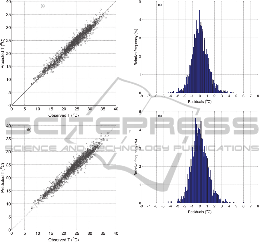
Figure 2: Comparison of the observed and predicted air

temperature values for the (a) MLPANN and (b)

RBFANN schemes.

3.3 Temporal Estimation of Air

Temperature

3.3.1 Implementation

For the temporal forecasting of air temperature

ANNs are used as function approximators aiming to

estimate the air temperature in a location using the

current and previous air temperature observations

from the same site.

In this application the Feed-Forward Artificial

Neural Network architecture with one hidden layer

is selected for predicting the air temperature time

series.

Figure 3: The residuals’ distribution for the (a) MLPANN

and the (b) RBFANN models.

Separate ANNs are trained and tested for predicting

the one hour (ANN-T1), two hours (ANN-T2) and

three hours (ANN-T3) ahead air temperature at

Airport station, based on the current and the five

previous air temperature observations from the same

site Therefore, the input in each ANN is the air

temperature at t, t-1, t-2, t-3, t-4 and t-5 and the

output is the air temperature at: t+1 for the ANN-T1,

t+2 for the ANN-T2 and t+3 for the ANN-T3.

The study period is from 19 July 2004 to 31

August 2006. In all cases, the first 60% of the

dataset is used for training the ANNs, the subsequent

20% for validation and the remaining 20% for

testing, as was described for the case of spatial

estimation of air temperature.

The optimum architecture (number of PEs in the

hidden layer) is related to the complexity of the

input and output mapping, along with the amount of

ICPRAM2013-InternationalConferenceonPatternRecognitionApplicationsandMethods

674

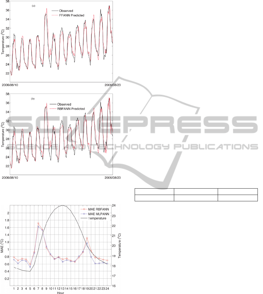
Figure 4: Comparison of the observed and predicted time

series for the (a) MLPANN and (b) RFBANN models.

Figure 5: Hourly MAE values and comparison with the

hourly temperature evolution and the Airport station.

noise and the size of the training data. A small

number of PEs result to a non-optimum estimation

of the input-output relationship, while too many PEs

result to overfitting and failure to generalize

(Gardner and Dorling, 1998). In this study the

selection of the number of PEs in the hidden layer is

based on a trial and error procedure and the

performance is measured using the validation set. In

each case, ANNs with a varying number from 5 to

25 PEs in the hidden layer were trained using the

Levenberg-Marquardt backpropagation algorithm

with the optimum architecture being the one that

minimizes the Mean Absolute Error (MAE) on the

validation set. A drawback of the backpropagation

algorithm is its sensitivity to initial weights. During

training, the algorithm can become trapped in local

minima of the error function, preventing it from

finding the optimum solution (Heaton, 2005). In this

study and for eliminating this weakness, each

network is trained multiple times (50 repetitions)

with different initial weights. A hyperbolic tangent

sigmoid transfer function tansig(n) = 2/(1+exp(-

2n))-1 was used as the activation function Ψ for the

PEs of the hidden layer. In the output layers, PEs

with a linear transfer function were used.

The optimum topologies of the selected ANNs

that minimized the MAE on the validation set are

presented in Table 3. In all cases, the architecture

includes six PEs in the input layer and one PE in the

output layer. The results indicate that the number of

the neurons in the hidden layer is increased as the

lag for forecasting the air temperature is increased.

Table 3: Optimum ANN architecture – number of PEs at

the input, hidden and output layer.

FFANN-T1 FFANN-T2 FFANN-T3

6 – 12 – 1 6 – 13 – 1 6 – 21 – 1

3.3.2 Results

The model evaluation statistics for the Airport

station are presented in Table 4 and the observed and

AAN based predicted air temperature values are

compared in the scatter plots of Figure 6. A general

remark is that the ANNs performance is decreased

with increasing the forecasting lag. In all cases the

MAE is less than 1.4 °C and the explained variance

decreases from 97.7% for the ANN-T1 to 88.7% for

the ANN-T3 model.

The ANN-T1 model exhibits very good

performance, as it is observed from the limited

dispersion along the optimum agreement line of the

one-hour air temperature (Figure 6a). The data

dispersion for the ANN-T2 (Figure 6b) and for the

ANN-T3 (Figure 6c) scatter plots is increased and a

small tendency of over-estimation of the low air

temperature values along with an under-estimation

of the high air temperature values is observed. This

finding is furthermore established from the increased

MBE for the ANN-T3 model

(°C).

ArtificialNeuralNetworkbasedMethodologiesfortheSpatialandTemporalEstimationofAirTemperature-Application

intheGreaterAreaofChania,Greece

675

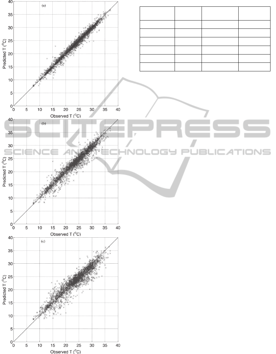
Figure 6: Comparison of the observed and ANN based

predicted air temperature values for the (a) one-hour, (b)

two-hour (b) and (c) three-hour ahead estimation.

Table 4: ANN based model performance.

FFANN

-T1

FFANN-T2

FFANN-

0.988

0.967 0.942

0.977

0.935 0.887

MBE (°C)

-0.068

-0.225 -0.405

MAE (°C)

0.589

0.996 1.361

RMSE (°C)

0.844

1.427 1.904

0.994 0.983

0.968

Regarding the residuals distributions (Figure 7), the

errors for the ANN-T1 and for the ANN-T2 are

approximately centered at 0 °C, while for the ANN-

T3 model the maxima of the distribution is shifted to

negative residual values, a fact which is attributed to

the tendency of the ANN-T3 model to underestimate

the air temperature values.

4 CONCLUSIONS

The ability of neural networks to spatial estimate

and predict short term air temperature values is

studied extensively and is well established. We

reviewed the theoretical background and the relative

advantages and limitations of ANN methodologies

applicable to the field of air temperature time series

and spatial modeling. Then, we have applied ANNs

methodologies in the case of a specific region with

complex terrain at Chania coastal region, Crete

island, Greece. Details of the implementation issues

are given along with the set of metrics for evaluating

the accuracy of the methodology. A number of

alternatives feed-forward ANN topologies have been

applied in order to assess the spatial and time series

air temperature prediction capabilities. For the one

hour, two hours and three hours ahead air

temperature temporal forecasting at a specific site

ANNs were trained based on the current and the five

previous air temperature observations from the same

site using the Levenberg-Marquardt back-

propagation algorithm with the optimum architecture

being the one that minimizes the Mean Absolute

Error on the validation set. For the spatial estimation

of air temperature at a target site the non-linear

Radial Basis Function and Multilayer Perceptrons

non-linear Feed Forward AANs schemes were

compared. The underlying air temperature temporal

and spatial variability is found to be modeled

efficiently by the ANNs.

ICPRAM2013-InternationalConferenceonPatternRecognitionApplicationsandMethods

676

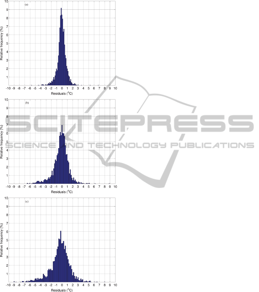
Figure 7: Comparison of the residuals distributions for the

(a) FFANN-T1, (b) FFANN-T2 and (c) FFANN-T3

models.

ACKNOWLEDGEMENTS

This research was partially funded by the University

of Athens Special Account for Research Grants.

REFERENCES

Bishop, C. M. (1995). Neural networks for pattern

recognition (1st ed.). Cambridge: Oxford University

Press.

Chai, H., Cheng, W., Zhou, C., Chen, X., Ma, X. & Zhao,

S. (2011). Analysis and comparison of spatial

interpolation methods for temperature data in Xinjiang

Uygur Autonomous Region, China. Natural Science,

3(12), 999-1010. doi:10.4236/ns.2011.312125.

Chronopoulos, K., Tsiros, I., Dimopoulos, I. & Alvertos,

N. (2008). An application of artificial neural network

models to estimate air temperature data in areas with

sparse network of meteorological stations. Journal of

Environmental Science and Health, Part A:

Toxic/Hazardous Substances and Environmental

Engineering, 43(14), 1752–1757. doi: 10.1080/

10934520802507621.

Cybenco, G. (1989). Approximation by superposition of a

sigmoidal function. Mathematics of Control Signals

and Systems, 2(4), 303–314. doi:

10.1007/BF02551274.

Deligiorgi, D., Kolokotsa, D., Papakostas, T., Mantou, E.

(2007). Analysis of the wind field at the broader area

of Chania, Crete. Proceedings of the 3rd

IASME/WSEAS International Conference on Energy,

Environment and Sustainable Development (pp 270-

275). Agios Nikolaos, Crete: World Scientific and

Engineering Academy and Society Press. Retrieved

from: http://www.wseas.us/e-

brary/conferences/2007creteeeesd/papers/562-194.pdf.

Deligiorgi, D., Philippopoulos, K. (2011). Spatial

Interpolation Methodologies in Urban Air Pollution

Modeling: Application for the Greater Area of

Metropolitan Athens, Greece. In F. Nejadkoorki (Ed.)

Advanced Air Pollution, Rijeka, Croatia: InTech

Publishers. doi: 10.5772/17734.

Deligiorgi, D., Philippopoulos, K., & Kouroupetroglou, G.

(2012, to appear). Artificial Neural Network based

methodologies for the estimation of wind speed. In F.

Cavallaro, F. (Ed.) Assesment and Simulation tools for

Sustainable energy Systems. Berlin: Springer.

Dombayc, O. & Golcu, M. (2009). Daily means ambient

temperature prediction using artificial neural network

method: A case study of Turkey. Renewable Energy,

34(3), 1158–1161. doi: 10.1016/j.renene.2008.07.007.

Fausett, L. V. (1994). Fundamentals neural networks:

architecture, algorithms, and applications. New

Jersey: Prentice-Hall, Inc.

Fox, D. G. (1981). Judging air quality model performance.

Bulletin of the American Meteorological Society,

62(5), 599–609. doi: 10.1175/1520-0477(1981)062<

0599:JAQMP>2.0.CO;2.

Gardner, M. W. & Dorling, S. R. (1998). Artificial neural

networks (the multilayer perceptron)-A review of

applications in the atmospheric sciences. Atmospheric

Environment, 32(14-15), 2627–2636. doi: 10.1016/

S1352-2310(97)00447-0.

Heaton, J. (2005). Introduction to Neural Networks with

Java. Chesterfield: Heaton Research Inc.

ArtificialNeuralNetworkbasedMethodologiesfortheSpatialandTemporalEstimationofAirTemperature-Application

intheGreaterAreaofChania,Greece

677

Hornik, K., Stinchcombe, M. & White, H. (1989).

Multilayer feedforward networks are universal

approximators. Neural Networks 2(5), 359–366. doi:

10.1016/0893-6080(89)90020-8.

Jain, A. K., Mao, J. & Mohiuddin, K. M. (1996). Artificial

neural networks: a tutorial. Computer 29(3), 31–44.

doi:10.1109/2.485891.

Koletsis, I., Lagouvardos, K., Kotroni, V. & Bartzokas,

A., (2009). The interaction of northern wind flow with

the complex topography of Crete island-Part 1:

Observational study. Natural Hazards and Earth

System Sciences, 9, 1845–1855. doi: 10.5194/nhess-9-

1845-2009.

Koletsis, I., Lagouvardos, K., Kotroni, V. & Bartzokas. A.

(2010). The interaction of northern wind flow with the

complex topography of Crete island-Part 2: Numerical

study. Natural Hazards and Earth System Sciences 10,

1115–1127. doi: 10.5194/nhess-10-1115-2010.

Kotroni, V., Lagouvardos, K. & Lalas, D. (2001). The

effect of the island of Crete on the etesian winds over

the Aegean sea. Quarterly Journal of the Royal

Meteorological Society 127(576), 1917–1937. doi:

10.1002/qj.49712757604.

Mihalakakou, G., Flocas, H., Santamouris, M. & Helmis,

C. (2002). Application of Neural Networks to the

Simulation of the Heat Island over Athens, Greece,

Using Synoptic Types as a Predictor. Journal of

Applied Meteorology, 41(5), 519-527. doi: 10.1175/

1520-0450(2002)041<0519:AONNTT>2.0.CO;2.

Mustafaraj, G., Lowry, G. & Chen, J. (2011). Prediction of

room temperature and relative humidity by

autoregressive linear and nonlinear neural network

models for an open office. Energy and Buildings,

43(6), 1452-1460. doi: 10.1016/j.enbuild.2011.02. 007

Powell, M. J. D. (1987). Radial basis functions for

multivariable interpolation: a review. Mason, J. C. &

Cox, M. G. (Eds) Algorithms for Approximation,

Oxford: Clarendon Press.

Price, D. T., McKenney, D. W., Nalder, I.A., Hutchinson,

M. F. & Kesteven, J. L. (2000). A comparison of two

statistical methods for spatial interpolation of

Canadian monthly mean climate data. Agricultural

and Forest Meteorology, 101(2-3), 81-94.

doi:10.1016/S0168-1923(99)00169-0.

Rumelhart, D. E., Hinton, G. E. & Williams, R. J. (1986).

Learning representations by back-propagating errors.

Nature 323, 533–536. doi: 10.1038/323533a0

Smith, B., Hoogenboom, G. & McClendon, R. (2009).

Artificial neural networks for automated year-round

temperature prediction. Computers and Electronics in

Agriculture 68(1), 52–61. doi: 10.1016/j.compag.

2009.04.003.

Snell, S., Gopal, S. & Kaufmann, R. (2000). Spatial

Interpolation of Surface Air Temperatures Using

Artificial Neural Networks: Evaluating Their Use for

Downscaling GCMs. Journal of Climate, 13(5), 886-

895. doi: 0.1175/1520-0442(2000)013<0886: SIOSAT

>2.0.CO;2.

Tasadduq, I., Rehman, S. & Bubshait, K. (2002).

Application of neural networks for the prediction of

hourly mean surface temperatures in Saudi Arabia.

Renewable Energy, 25(4), 545–554. doi: 10.1016/

S0960 -1481(01)00082-9.

Willmott, C. J. (1982). Some comments on the evaluation

of model performance. Bulletin American

Meteorological Society, 63(11), 1309–1313. doi: 10.

1175/1520-0477(1982)063<1309:SCOTEO>

2.0.CO;2.

Yu, H. & Wilamowski, B. M. (2011). Levenberg–

Marquardt training. Wilamowski, B.M. & Irwin, J.D.

(Eds) Industrial Electronics Handbook (2nd ed.). Boca

Raton: CRC Press.

Zhang, G. P., Patuwo, E. & Hu, M. (1998). Forecasting

with artiﬁcial neural networks: the state of the art.

International Journal of Forecasting, 14(1), 35–62.

doi: 10.1016/S0169-2070(97)00044-7.

ICPRAM2013-InternationalConferenceonPatternRecognitionApplicationsandMethods

678