Simple Gestalt Algebra
Eckart Michaelsen
1
and Vera V. Yashina
2
1
FhG-IOSB, Gutleuthausstrasse, 1, 76275 Ettlingen, Germany
2
Dorodnicyn Centre RAS, 40, Vavilov str., Moscow, Russia
Abstract. The laws of Gestalt perception rule how parts are assembled into a
perceived aggregate. This contribution defines them in an algebraic setting.
Operations are defined for mirror symmetry and repetition in rows respectively.
Deviations from the ideal case are handled using positive and differentiable as-
sessment functions achieving maximal value for the ideal case and approaching
zero if the parts mutually violate the Gestalt laws. Practically, these definitions
and calculations can be used in two ways: 1. Images with Gestalts can be ren-
dered by using random decisions with the assessment functions as densities; 2.
given an image (in which Gestalts are supposed) Gestalt-terms are constructed
successively, and the ones with high assessment values are accepted as plausi-
ble, and thus recognized.
1 Introduction
The Gestalt Algebra is meant to capture the laws of perception – as unveiled e.g. by
Wertheimer [10] – in a formal way. Thus the algebraic nature of perceived gestalts
can be soundly described and in the end coded on machines. A gestalt is always an
aggregate composed of its parts. It means more, but is completely determined by its
parts. With universal algebra there is a sound apparatus for capturing these ideas with
more rigors.
1.1 Related Work
The notion of a maximum-meaningful gestalt is due to A. Desolneux [2] referring to
statistical models for background clutter and foreground gestalts much similar to the
ones discussed here. She actually refers again to D. Love, D. Marr and even H. von
Helmholtz. Above we already mentioned the pioneering work of Wertheimer.
The universal algebra (for which our definitions below are a special case) has been
thoroughly investigated by A. I. Malcev [4]. Here operations are allowed with more
than 0, 1, or 2 aryties. Such algebras are called homogenous, as long as they work
only on one common set. Bikhoff & Lipson [1] generalize to heterogeneous algebras
working on several sets (called phylae) in order to include things like modules, vec-
tor-spaces, etc. An important specialization of that for image generation, understand-
Michaelsen E. and V. Yashina V..
Simple Gestalt Algebra.
DOI: 10.5220/0004393300380047
In Proceedings of the 4th International Workshop on Image Mining. Theory and Applications (IMTA-4-2013), pages 38-47
ISBN: 978-989-8565-50-1
Copyright
c
 2013 SCITEPRESS (Science and Technology Publications, Lda.)

ing, and mining is the Ritter image algebra [8, 9]. A very sophisticated pattern algebra
with generators and connectors has been defined by Grenander [3]. Own previous
work – however rather informal, lacking proven results – has been published in [6, 7].
2 Definition of the Simple Gestalt Algebra
First the Gestalt space will be defined. Then two operations (|and ∑) will be given,
constructing new elements from given ones. While | is a binary operation, ∑ is of
unspecified arity. Closure will be proven, i.e. that all operations lead to well defined
new elements of the Gestalt space. Thus the Gestalt algebra is a special form of a
universal algebra in the Malcev sense. But we neither give neutral elements nor the
projections, as is usually done in Algebra. Also inverse elements are not possible.
2.1 Gestalt Space
The product set


2
mod (0, ) [0,1]G   
(1)
will be regarded as Gestalt space (of the plane). For each gєG the first component is
called its position po(g)є R
2
; the second component is called its orientation or(g)є R
mod π; the third component is called its scale sc(g)>0; the fourth component is called
its assessment 0≤as(g)≤1. The Gestalt space obviously is a smooth manifold with
boundaries. Figure 1 shows some random instances of the gestalt space. They are
depicted in a grey-tone according to their assessment with white meaning assessment
zero and black meaning assessment one. Uniform random attributes where chosen
with position from [0,10]× [0,10], scale from (0,3], and assessment from [0,1] re-
spectively.
2.2 Forming a Mirror Gestalt from two Parts
Definition 1: (Mirror operation). The binary operation | is defined as
 
|
1
| () (), () (),| () ()| () (), ,
2
g
h po g po h ori po g po h po g po h sc g sc h a g h

  


.
(2)
The position of the new Gestalt results from averaging the positions of its parts. The
orientation of the new Gestalt is a function ori of a 2D vector v. It is obtained by
ori(v)=arctan(v
y
/v
x
) for v
x
≠0 and set to π/2 if v
x
=0. The new scale is the sum of the
Euclidean distance between the positions of the first and second part plus the geomet-
ric mean of the two scales. The assessment a
|
is a geometric mean of a product of four
partial assessments:
39

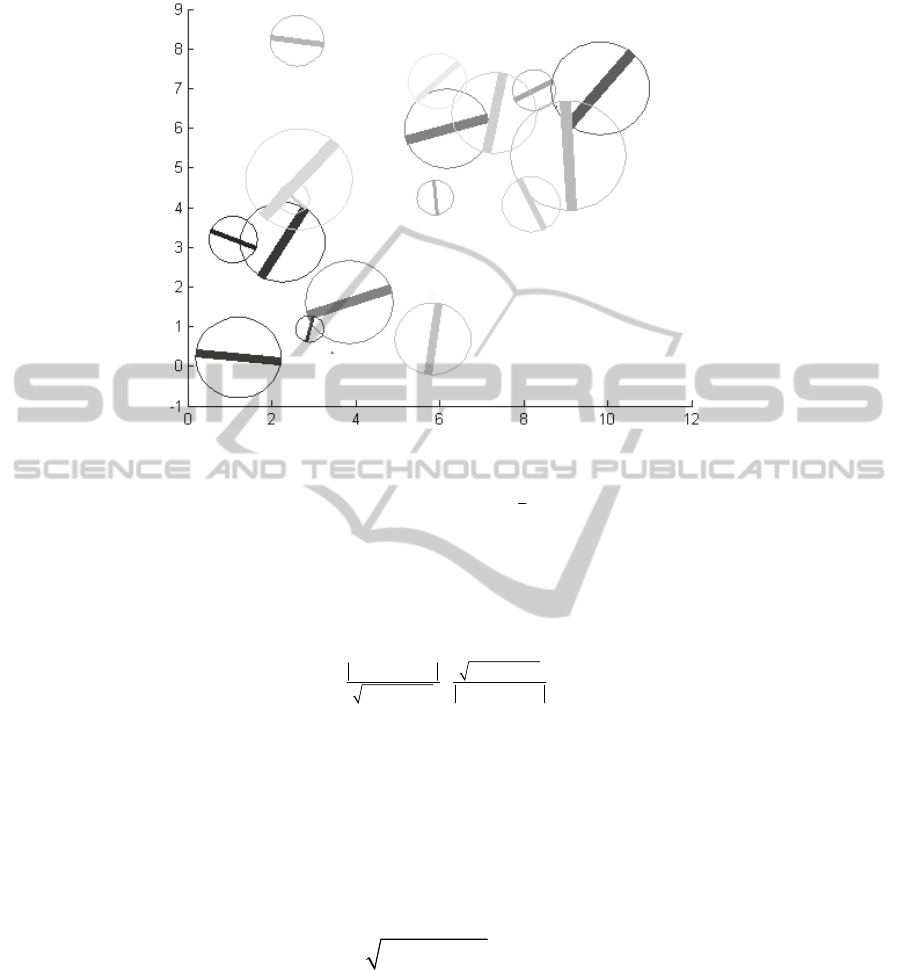
Fig. 1. A set of 20 randomly chosen gestalts.


1
4
||,|,|,|,
,
posa
agh a a a a
.
(3)
Before we give the definitions of these partial assessment functions let us consider the
properties of two important help functions namely the perceptual attention function
exp(2-x-1/x) on x>0 and the angular neighbor function α=½+½cos(2x) on 0≤x<π as
they are displayed in Figure 2.
() ()
() ()
2
() ()
() ()
|,
po g po h
s
cgsch
po g po h
sc g sc h
p
ae




,
(4)
has thus the form of a perceptual attention, and if a denominator in (4) should be zero
we may set continuously a
|,p
=0.


|,
() () 2 ( |)
o
a org orh org h  
, where α is the angular neighborhood.
(5)
2 ()/ () ()/ ()
|,
s
c h sc g sc g sc h
s
ae


(also a perceptual attention),
(6)
and another geometric mean
|,
() ()
a
aasgash
.
(7)
Figure 3 shows examples of the operation at work. Actually, the small black part
gestalts were generated using the method sketched in section 3.1.: 1) pick a random
common orientation for the parts uniformly from [0, π); 2) disturb the position, scale,
and orientation attributes according to the є value chosen. With rising є the new ge-
stalt (depicted in grey) will get a lower assessment (depicted as brighter grey).
40

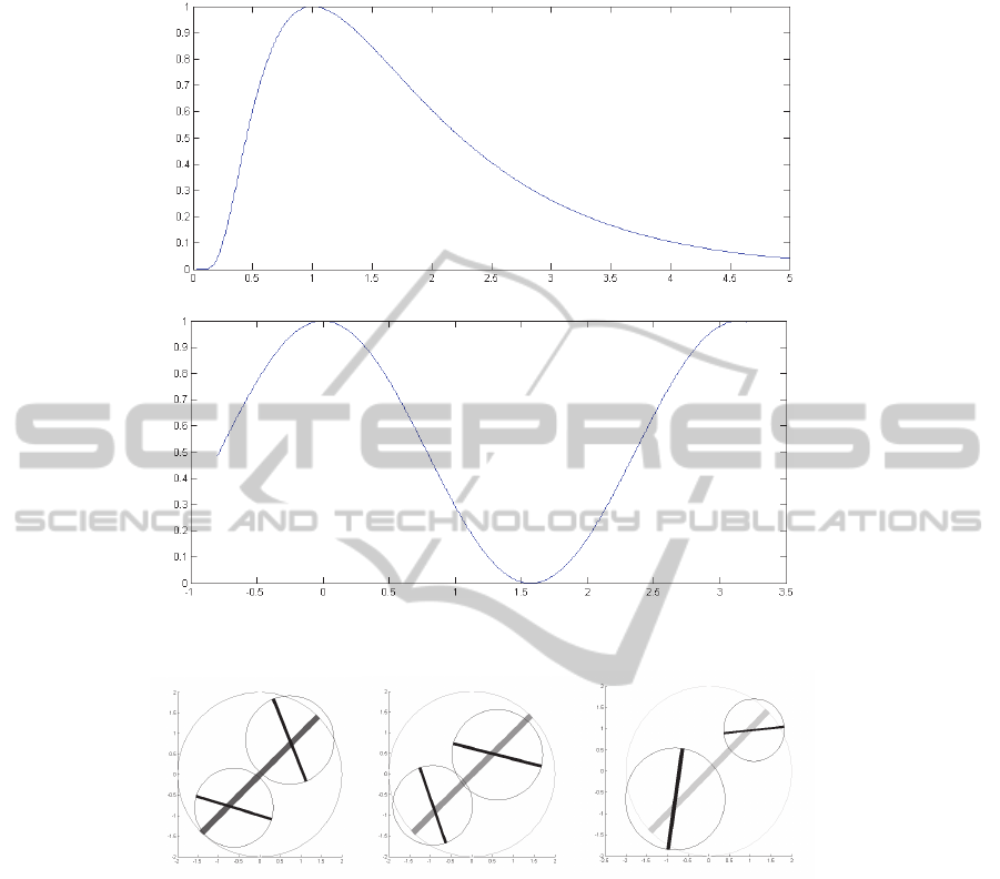
Fig. 2. Auxiliary functions for gestalt assessment calculation: Upper, perceptual atten-
tion;lower, angular neighborhood α.
Fig. 3. Three terms of the mirror operation with left-to-right declining assessment
(є=0.05,0.1,0.2).
Theorem 1. (Closure) g|h є G for any g, h є G. Proof: 1) Position attribute: The aver-
age position of two points of R
2
is in R
2
. 2) Orientation attribute: Arctangent yields
always an orientation value modulo π. Moreover, for v
x
→0 we have ori→± π/2, so
the function ori is smooth except for v
x
=v
y
=0. This occurs e.g. for g=h; still also for
these cases the orientation value is defined. 3) Scale attribute: Both, the absolute
value, as well as the root, are positive, so is the sum of an absolute value and a root.
4) Assessment attribute: We shall prove that all four functions a
|,p
, a
|,o
, a
|,s
, a
|,a
, є [0,1]
then the geometric mean (3) will also be there: a
|,p
and a
|,s
are functions of the form
exp(2-x-1/x); it is easily verified that this positive function takes its maximum value 1
for x=1; for x→0,∞ this function approaches zero (and thus is smooth everywhere,
41

see also Fig. 2); for a
|,o
consider (5) where some operations inside the orientation
attribute are performed, which is a group with respect to addition; the function α is
bounded between zero and one; a
|,a
is again a geometric mean of values from [0,1].□
Lemma 1. (Commutativity) g|h=h|g for any g, h. Proof: By checking symmetry of
definitions and function ori. □ Note, that interchanging g and h can be interpreted as
operation of the trivial two member group.
Lemma 2. (Self is worst) as(g|g)=0 for any g. Proof: By checking (4) we find a
|,p
=0
for this case and thus a zero in the product (3).□
Remark 1. a
|,p
=1 if |p(g)-p(h)| equals the geometric mean of s(g) and s(h); else it will
be smaller. If they are much further away of each other or much closer a
|,p
will ap-
proach zero. A deviation of some factor t >1 causes the same punishment as a corre-
sponding deviation of factor 1/ t.
Remark 2. The orientation assessment function α gives α(0)= α(π)=1 and α(π/2)=0;
so according to (5) a
|,o
=1 iff the orientations are mirror symmetric to each other with
respect to or(g|h). This is why we call this operation “mirror operation”. See also
Figure 3 for examples of assessment better 1- є.
Lemma 3. (Monotonicity) (sc(g)·sc(h))
1/2
≤ sc(g|h) for any g, h. Proof: By checking
(2) and because absolute values are positive.□
2.3 Summation into Row Gestalts
Definition 2: (Mirror operation). The operation ∑ is of arity n>1. It is defined as

1
1111
1
1
... ( ), ( ) ( ) , | ( ) ( ) |, ,...,
n
ni iimidn n
i
g
g pog ori pog pog sc pog pog a g g
n











.
(8)
So the position of the new Gestalt results from averaging the positions of its parts.
The orientation of the new Gestalt is obtained from summing up the difference vec-
tors of the positions, where the function ori of a 2D vector v is again obtained by
ori(v)=arctan(v
y
/v
x
) provided that v
x
≠0 and ori= π/2 else. The new scale is obtained
from the Euclidean distance between the positions of the first and the last part plus
the geometric mean of the scales sc
mid
=(sc(g
1
)…sc(g
n
))
1/n
. The assessment is again a
geometric mean of a product of four partial assessments


1
1,,,,
,...,
n
nposa
ag g a a a a


,
(9)
Where the positioning assessment is acquired as deviation from set-positions as
42

1
()
()
,
1
ii
i
po g set
n
n
sc g
p
i
ae










with






1
11
1
cos ...
(1)/2
... ...
1
sin ...
n
inn
n
or g g
in
set p g g s g g
n
or g g



   




(10)
and we make use again of assessing angular differences by function α of (4) setting

1
,1
1
( ) ( ... )
n
n
oin
i
aogavogg 







,
(11)
Here the average orientation avo is obtained by summing up all orientations (as unit
vectors) and using ori from (7). This can be problematic if the sum should equal zero.
11
(2 ... 1/ ... 1/ )/
,
nn
nt t t t n
s
ae
  


, where t
i
=sc(g
i
)/sc
mid
(12)
and sc
mid
is again the geometric mean of the scales, and also

1
,1
( ) ... ( )
n
an
aagag


.
(13)
Figure 4 shows examples of the operation at work. Actually, the small black part
gestalts were generated using the method sketched in section 3.1.: 1) Specify how
many parts are to be built (in this case 5). From this follows the set-positions and the
common scale of the parts; 2) pick a random common orientation for the parts uni-
formly from [0, π); 3) disturb the position, scale, and orientation attributes according
to the є value chosen. With rising є the new gestalt (depicted in grey) will get a lower
assessment (depicted as brighter grey).
Fig. 4. Three terms of the row operation with left-to-right declining assessment
(є=0.05,0.1,0.2).
Theorem 2. (Closure) ∑g
1
…g
n
є G for any g
1
…g
n
є G. Proof: 1) Position attribute:
The average position of n points of R
2
is in R
2
. 2) Orientation attribute: Arctangent
yields always an orientation value modulo π (see part 2 of proof of theorem 1). 3)
Scale attribute: Both, the absolute value as well as the root are positive, so is the sum
of an absolute value and a root. 4) Assessment attribute: We shall prove that all four
functions a
∑,p
, a
∑,o
, a
∑,s
, a
∑,a
є [0,1] then the geometric mean (9) will also be there:
a
∑,p
is a product of functions of the form exp(-x) where 0≤x and thus bounded by zero
and one; a
∑,o
is a geometric mean of values obtained by function α and thus bounded
43

between zero and one; a
∑,s
is obtained from (12) which may be decomposed into a
product of n factors of form (4); a
∑,a
is again a geometric mean of values from [0,1].□
Lemma 4. (Generalized commutativity) ∑g
n
…g
1
=∑g
1
…g
n
for any g
1
,… g
n
. Proof:
By checking symmetry of definitions and function ori. □ Note, the index mappings
{i→i, i→n+1-i} are a sub-group of the group of index permutations.
Lemma 5. (Self is worst) as(∑g…g)=0 for any g. Proof: By checking (10) we find
a
∑,p
=0 for this case and thus a zero in the product (3).□
Lemma 6. (Monotonicity) (sc(g
1
)·… ·sc(g
n
))
1/n
≤ sc(∑g…g) for any g
1
…g
n
. Proof: By
checking (8) and because absolute values are positive.□
3 Some Useful further Definitions and Results
For a small ε>0, we may define the relation =
ε
by g=
ε
h iff |as(g)- as(h)|<ε and the
other attributes of g and h are equal. Then we get
Lemma 7. For any small ε>0 exists a small angle δ such that for any g and h
g|h=
ε
∑gh if |or(g)-or(g|h)+π/2|<δ and |or(h)-or(g|h)+π/2|<δ. Proof: Comparing (2)
and (8) we find po(g|h)=po(∑gh), or(g|h)=or(∑gh), and sc(g|h)=sc(∑gh) respective-
ly. The same holds for the assessment components: (4) equivalent to (10), (6) equiva-
lent to (12), and (7) equivalent to (13). The only difference is in (5) versus (11). But
for |or(g)-or(g|h)+π/2|<δ and |or(h)-or(g|h)+π/2|<δ we will have both a
∑ ,p
>1- ε and
a
| ,p
>1- ε.□
Recall here that for small angles δ the cos(δ ) can be approximated as 1. So for very
small ε>0, δ may be a considerable deviation. We will always have particular interest
in such cases, where the same parts arranged differently in a term still yield the same
(or ε-same) gestalt object:
Definition 3: (Gestalt equivalence). We define a gestalt-term recursively: 1) Each
gєG is a term. 2) For two terms s and t s|t is a term as well as for n terms t
1
…t
n
∑t
1
…t
n
is a term. Interchanging s and t as well as reordering t
1
…t
n
into t
n
…t
1
does not change
the value of the term in gestalt space (Lemmata 1 and 4). Thus there is an equivalence
relation defined on the set of gestalt-terms. The corresponding equivalence classes are
the main objects of our interest (gestalts).
44

Definition 4: (Search regions). For gєG and ε>0 the set {hєG; ass(g|h)>1- ε} is
called ε-mirror-search-region; For g
i
єG , 0<i≤n, and ε>0 the union of sets




1
; ... 1
jn
ji
gGas gg





(14)
is called ε-i-n-row-search-region.
4 Gestalt Algebra at Work
We state that only gestalts with high assessments are meaningful. Thus the margin of
the manifold, where as(g)=1, is of most interest. Close to this margin, i.e. where
as(g)=1-є with a small є >0, only small deviations from the ideal gestalt laws occur.
Two possible utilizations are possible: Generative and reducing.
4.1 Generating Gestalts
One or more large Gestalts are set by a user filling the screen (or sheet). Then recur-
sively each Gestalt is decomposed by: 1) Choosing randomly an operation from | and
∑ and (if it is not |) an arity n; 2) Choosing decompositions accordingly and at ran-
dom such that the (normed) assessment functions are used as densities for drawing
the new positions, orientations, and scales, respectively. To this end the integrals of
the assessment functions over the whole admissible domain must be finite, so that
they can be normed using the inverse of the integral as factor. Then they can be used
as probability density functions for the random choice.
From Lemmas 3 and 6 it follows, that the Gestalts thus generated will become
smaller and smaller. The generation may be terminated if they are smaller than a
threshold (e.g. 5 Pixel). Then all these Gestalts can be drawn rendering an image. If
the random numbers are not newly drawn for each branch of the term tree, but instead
copied from one branch to the other, the image will exhibit interesting symmetries.
4.2 Reducing Gestalts
Primitive gestalts of small size are obtained from a digital image. The simplest way is
using one of the commonly used edge detection methods. They are assessed e.g. ac-
cording to the gradient magnitude. Position and orientation are also naturally given.
The scale is fixed and obtains the same value for all primitives (such as two or three
pixel). Another possibility is using the well-known SIFT method. It naturally sets the
position, orientation, scale and assessment attributes for each extracted feature (i.e.
primitive gestalt).
Then the gestalts are successively and at random combined into new gestalts.
Again the assessment functions are used for drawing with preference. A suitable
interpretation system for doing so has also been given by [5]. In the end terms of the
45

Gestalt Algebra are reduced from images. They may be visualized as reduction trees.
Each such term has an assessment. For such procedure Definition 2 is of high interest,
since equivalent terms may be reduced on different branches of the search. In order to
avoid combinatorial explosion with the size of the terms, it is important to store the
terms as representatives of the equivalence classes, and avoid multiple storage.
Drawing with preference means that the interpreter works on a set of existing ge-
stalts. It selects better assessed ones with higher probability. Then it looks for suitable
partners to form new gestalts using the three gestalt operations. “Suitable” here means
it queries the set for partners such that the resulting gestalts have assessment 1-є with
a small є >0. Search regions in the gestalt space can be constructed by fixing є and
setting the derivative of the assessment function zero.
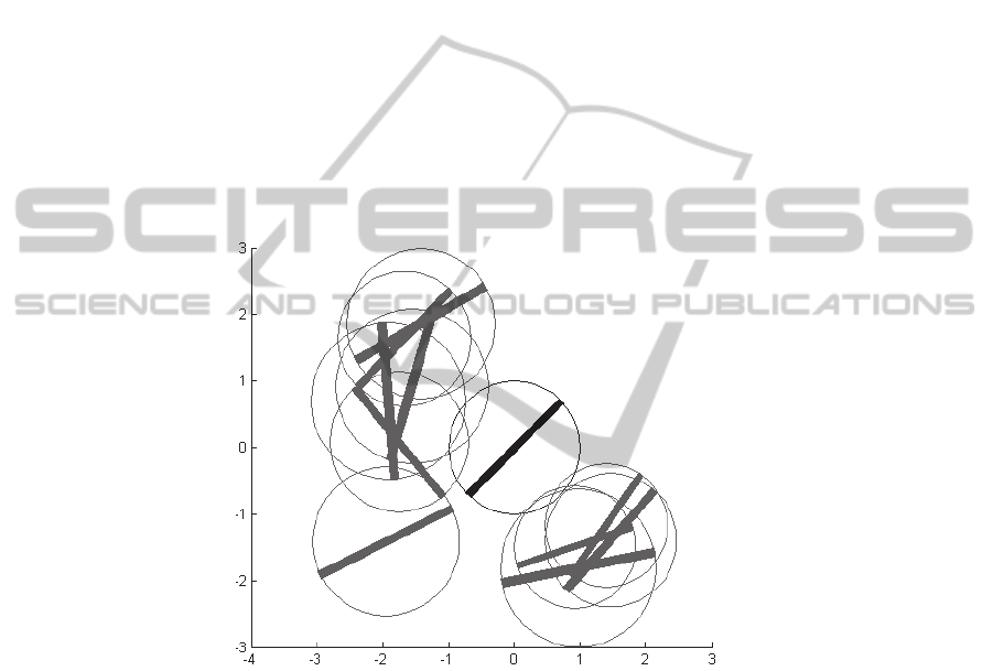
Figure 4 illustrates this: One gestalt g is displayed in the middle and possible part-
ners h arranged around it such that the components of the assessment function are
better than 1-є. Possible partner gestalts are of about the same size, and in appropriate
distance. The search region for the position is bounded by two concentric circles
around g. Most important: Their orientation roughly fits the mirror symmetry con-
straint.
Fig. 5. A gestalt (black) and a set of 10 randomly chosen partner gestalts (grey) with position,
scale and orientation attributes in the 1-є domain (є=0.1).
5 Discussion, Outlook, and Conclusions
We have presented an algebraic setting for the laws of gestalt perception. With such
definitions, lemmas and theorems at hand the endeavor of machine coding such per-
ceptive capabilities, as they are found in e.g. human subjects, will be facilitated.
Much work lies still ahead:
46

5.1 Product into Rotational Mandalas
In [7] an operation ∏ was defined of arity n>1. For a good assessment the parts
should be arranged in a regular polyhedron with n vertices. An iterative solution was
given (equation (4)) for the attributes po and sc, fitting quite perfectly into the settings
here. The position of the new Gestalt is initialized by averaging the positions of its
parts. The radius of the polyhedron can be initialized from the mid distance of the
parts to the initial position. A closure theorem would have to prove the convergence
of the iteration.
We did not (yet) include this operation here, because there is a problem with the
orientation attribute: The iteration outlined in [own citation] yields a phase defined in
[0,2π/n). This does not really fit the intentions of the second component of G in (1).
The operation would be of interest, for instance because an interesting Lemma on
generalized commutativity could be stated here stating ∏g
1
…g
n
=∏g
σ(1)
…g
σ(n)
for any
σ
є D
n
where D
n
is the Dihedral group of n. So here we have non-trivial group action
on the gestalts. We will investigate this further and modify the definitions such that
this operation can also be included consistently.
References
1. Birkhoff G., Lipson J. D.: Heterogeneous Algebras. Journal of Combinatorial Theory,
Vol.8, 1970. pp. 115-133.
2. Desolneux A., Moisan L., Morel J.-M.: From Gestalt Theory to Image Analysis. Springer,
Berlin, 2008.
3. Grenander U.: General Pattern Theory. Oxford Science Publications, 1994.
4. Malcev A. I.: Algebraic Systems. Nauka, Moscow, 1970; Springer, Berlin, 1973.
5. Michaelsen E., Doktorski L., Luetjen K.: An Accumulating Interpreter for Cognitive Vi-
sion Production Systems. Pattern Recognition and Image Analysis, 2012, Vol. 22, No. 3,
pp. 464–469.
6. Michaelsen E., Meidow J.: Basic Definitions and Operations for Gestalt Algebra. In:
Gourevich I., Niemann H., Salvetti O. (eds.): IMTA 2009 – Image Mining Theory and
Applications. Lisbon, 2009. pp. 53-26.
7. Michaelsen E.: On the Construction of Gestalt-Algebra Instances and a Measure for their
Similarity. In: Gurevich I., Niemann H., Salvetti O. (eds.): IMTA 2010 – Image Mining
Theory and Applications. Angers, May 2010. pp. 51-59.
8. Ritter G. X.: Image Algebra. Online at: http://www.cise.ufl.edu/~jnw/CVAIIA/ (accessed
30.12.2012), 1993.
9. Ritter G. X., Wilson J.N.: Handbook of Computer Vision Algorithms in Image Algebra, 2-
d Edition. CRC Press Inc., 2001.
10. Wertheimer M.: Untersuchungen zur Lehre der Gestalt, II. Psychologische Forschung, Vol.
4 , 1923. pp. 301-350.
47