
Fuzzy-weighted Pearson Correlation Coefficient for Collaborative
Recommender Systems
Mohammad Yahya H. Al-Shamri and Nagi H. Al-Ashwal
Electrical Engineering Department, Faculty of Engineering and Architecture, Ibb University, Ibb, Yemen
Keywords: Collaborative Recommender Systems, Correlation Coefficient, Fuzzy Weighting.
Abstract: Memory-based collaborative recommender system (CRS) computes the similarity between users based on
their declared ratings. The most popular similarity measure for memory-based CRS is the Pearson
correlation coefficient which measures how much the two users are correlated. However, not all ratings are
of the same importance to the user. The set of ratings each user weights highly differs from user to user
according to his mood and taste. This will be reflected in the user’s rating scale. Accordingly, many efforts
have been done to introduce weights to Pearson correlation coefficient. In this paper we propose a fuzzy
weighting to the Pearson correlation coefficient which takes into account the different rating scales of
different users so that the rating deviation from the user’s mean rating is fuzzified not the rating itself. The
experimental results show that Pearson correlation coefficient with fuzzy weighting outperforms the
traditional approaches.
1 INTRODUCTION
Web services grow very fast letting Web users in a
difficult position to select from a huge number of
choices. Web personalization tools, especially
recommender systems (RS) help Web users navigate
Web easily and in a personalized way. The most
successful recommender system is the collaborative
recommender system (CRS) which recommends
items people with similar tastes and preferences
liked in the past to a given active user.
Formally, CRS have users,
,…,
,
rating explicitly or implicitly items, S
s
,…,s
, such as news, web pages, books, movies,
or CDs. Each user
has rated a subset of items
.
The declared rating of user u
for an item
is
denoted by r
,
(Goldberget al., 1992; Schafer et al.,
2007; Burke, 2002; Adomavicius and Tuzhilin,
2005) and the user’s average rating is denoted by
m
. To do its job, a memory-based CRS matches the
active user to the available database according to a
suitable similarity measure. The similarity between
two users is a measure of how closely they resemble
each other. Once similarity values are computed, the
system ranks users according to their similarity
values with the active user to extract a set of
neighbors for him. According to this set of
neighbors, the CRS assigns a predicted rating to all
the items seen by the neighborhood set and not by
the active user (Adomavicius and Tuzhilin, 2005).
The predicted rating,
,
, indicates the expected
interestingness of the item s
to the user u
.
The similarity computation phase for any RS
plays an important rule for the RS success. Different
similarity functions often leads to different sets of
neighbors for a given active user. A good similarity
function will be that one produces a close set of
neighbors for a given active user. The existing
similarity measures for memory-based CRS based
their work on the users’ raw declared ratings or on
the deviation of these ratings from the users mean
ratings. However, the users’ tastes for ratings differ
from time to time and the actual employed rating
scale differs from user to user. Therefore the raw
declared users’ ratings need to be weighted so that a
weighted rating scale is obtained for all users.
Most of the previous work was focusing either
on genetic algorithm (GA) to evolve weights
(Bobadilla et al., 2011; Min and Han, 2005) or on
trust and reputation as similarity modifiers for the
existing Pearson correlation coefficient (Bharadwaj
and Al-Shamri, 2009). However, GA approach takes
a long time for training and requires the system to
store the evolved weights which is an extra load for
the system. In this paper we propose a fuzzy
409
Yahya H. Al-Shamri M. and H. Al-Ashwal N..
Fuzzy-weighted Pearson Correlation Coefficient for Collaborative Recommender Systems.
DOI: 10.5220/0004412404090414
In Proceedings of the 15th International Conference on Enterprise Information Systems (ICEIS-2013), pages 409-414
ISBN: 978-989-8565-59-4
Copyright
c
2013 SCITEPRESS (Science and Technology Publications, Lda.)

weighting to the Pearson correlation coefficient.
This weighting will increase the effectiveness of the
correlation-based RS (CBRS) without loading it in
time or in space. Thus a close set of neighbors is
obtained which will increase the system accuracy.
The rest of this paper is organized as follows: an
introduction to some similarity measures for
memory-based CRS is given in Section 2. Fuzzy-
weighted Pearson correlation coefficient for CRS is
introduced in Section 3. Section 4 presents the
experimental results for the proposed approach with
the traditional approaches. Finally, we conclude our
work in the last section.
2 SIMILARITY MEASURES FOR
MEMORY-BASED
COLLABORATIVE RS
The most popular similarity function for memory-
based CRS is the Pearson correlation coefficient
(Burke, 2002; Adomavicius and Tuzhilin, 2005),
where the similarity between two users is computed
only based on the common ratings, S
, both users
have declared. The Pearson correlation coefficient
(PCC) is:
,
∑
,
,
∈
∑
,
2
∑
,
2
∈
∈
(1)
where
,
,
. The literature describes
also the cosine similarity measure (Adomavicius and
Tuzhilin, 2005), which treats each user as a vector in
the items’ space and then finds the cosine of the
angle between the two vectors.
,
∑
,
,
∈
∑
,
∑
,
∈
∈
(2)
Recently, Bobadilla et al., (2011) proposed the
mean difference weights similarity measure. This
similarity measure gets the average of the weights of
the ratings differences between the two users. These
weights are evolved using GA; however, they can be
assumed fixed to the mean of each difference weight
interval that have been proposed in (Bobadilla et al.,
2011). For our experiments, we set the weights fixed
to
1,0.5,0,0.5,1.
,
∑
,
,
∈
(3)
Bobadilla et al., (2011) divide Formula (3) by the
difference between the maximum and minimum
values of the rating scale. However, this factor is not
necessary because Formula (3) already divides the
weights by their number. The numerator cannot
exceed S
in any way since ∈1,1. The only
effect this factor has is reducing the similarity values
which in turn will reduce the contribution of each
neighbor’s rating in the aggregation process.
3 FUZZY-WEIGHTED PEARSON
CORRELATION COEFFICIENT
Weighting user ratings is an effective way to capture
the users’ different tastes for ratings scale. However,
most of the previous work based this weighting on
GA as a learning technique which is a good way if
we have time and space. Even GA can focus on the
good items while removing bad ones or reducing
their impacts but it requires a long time for learning
the weights and a large space for storing them.
Moreover, these weights have to be recalculated
periodically to capture the users changing tastes over
time.
A simple and effective way to alleviate the GA
difficulties will be that one uses fuzzy logic to get
the rating weights by employing the ratings
themselves. However, this will suffer from the
different users’ rating scales. Not all users use the
rating scale similarly; some users rate an item by 3
as bad item while others rate the same item by 3 as
good item. Thus instead of employing direct ratings
for evolving fuzzy weights, we can fuzzify the rating
deviation from the user’s mean ratings,
,
. This
will avoid the different rating scales problem. The
fuzzy-weighted Pearson correlation coefficient will
be as follow:
,
∑
,
,
∈
∑
,
∑
,
∈
∈
(4)
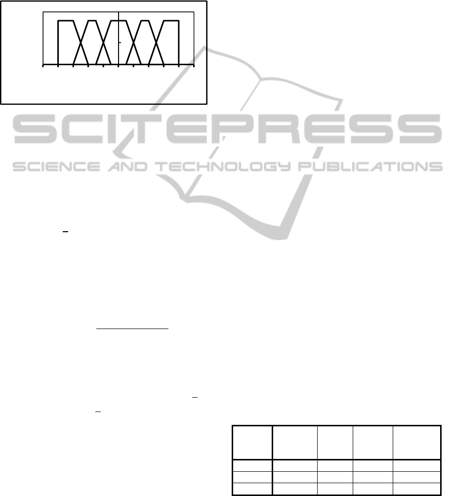
To fuzzify dev
,
., we define five fuzzy sets for
each deviation value (Figure 1). The membership
values for these fuzzy sets are defined as below:
1 43
0 42
2 32
(5a)
0 30.5
3 32
121.5
0.5 1.50.5
(5b)
0 1.51.5
1.5 1.50.5
1 0.50.5
1.5 0.51.5
(5c)
ICEIS2013-15thInternationalConferenceonEnterpriseInformationSystems
410
00.53
0.5 0.51.5
1 1.52
3 23
(5d)
024
1 34
2 23
(5e)
Figure 1: Fuzzy sets and their membership values for the
deviation values.
Accordingly, each deviation value will get a 5-
tuple membership values (5-tuple vector) to these
five fuzzy sets. For example, if
,
2.3, then
the corresponding 5-tuple membership vector will be
,
0,0,0,0.7,0.3. Based on the
membership vectors, we can get the fuzzy weighting
for the k
common item as:
√
2
,
,
,
(6)
where
,
is the membership vector for
,
value and
,
,
,
is any vector distance
metric. In this paper, Euclidean distance function is
used for computing disdev
,
,dev
,
. In general
,
and
,
are two vectors of size (in this
paper l5 ).
,
,
,
,
,
(7)
where dev
,
is the membership value of the dev
,
value to its j
fuzzy set [Al-Shamri & Bharadwaj,
2008]. We subtract disdev
,
,dev
,
from
√
2 in
Formula (6) because
√
2
is the maximum distance
value that we can get from Formula (7) [in this case
the two deviation values are belonging to two
different fuzzy sets with a unity membership value
to each one of them, for example
,
1,0,0,0,0 and
,
0,0,0,1,0].
4 EXPERIMENTS
We conduct our experiments using the one million
MovieLens (http://www.movielens.umn.edu, Dec
2012) dataset. This dataset consists of 1000209
ratings by 6040 users on 3900 movies. Table 1
illustrates the distribution of this dataset’s users
according to the number of each user’s declared
ratings.
The total dataset is divided into three datasets,
DataSet1, DataSet2, and DataSet3 according to each
user’s total ratings. We randomly select 500 users
out of 6040 users such that 50% (250 users) are
selected from DataSet1, 40% (200 users) are
selected from DataSet2, and 10% (50 users) are
selected from DataSet3. Keeping in mind the actual
users’ distribution, we subdivide the resulting
dataset into 10 mutually exclusive folds, fold(1), …,
fold(10), each of which having the same size, 50
users (25 users from DataSet1, 20 users from
DataSet2, and 10 users from DataSet3). Thus each
fold mimics the whole dataset distribution.
Training and testing are performed 10 times
where in iteration-i, fold(i) is reserved as the test set
and the remaining folds are collectively used to train
the system. That is in Split-1 dataset, fold(2),…,
fold(10) collectively serve as the training set while
fold(1) is the test users; Split-2 is trained on fold(1),
fold(3), …, fold(10) and tested on fold(2); and so on
(Han & Kamber, 2006). Thus each fold is used the
same number of times for training and once for
testing. Thus the number of total users, training
users, and active users are 500 ,
450 , and
50, respectively. During the testing phase, the
set of declared ratings,
, by an active user,
, are
divided randomly into two disjoint sets, namely
training ratings
(34%) and test ratings
(66%) such that
∪
. The RS treats
as the only declared ratings while
are treated as
unseen ratings that the system would attempt to
predict for testing the RS performance.
Table 1: The one million Movielens dataset users’
distribution.
DataSet
No.of
Users’
Ratings
No.of
Users
Total
Ratings
Percentage
(%)
DataSet1 20‐‐100 3154 155677 52
DataSet2 101‐‐500 2491 550580 41
DataSet3 >500 395 287913 7
To test the effectiveness of our approach, we
conduct four experiments on the 500 users’ dataset,
0
0,5
1
‐5 ‐4 ‐3 ‐2 ‐1012345
MembershipValue
DeviationValue
Fuzzy-weightedPearsonCorrelationCoefficientforCollaborativeRecommenderSystems
411

the first experiment uses Pearson correlation
coefficient (Formula (1)) for the similarity
computation and we call it Correlation-Based RS
(CBRS). The second experiment uses Cosine Vector
similarity measure (Formula (2)) for the similarity
computation and we call it Cosine Vector RS
(CVRS). The third experiment uses mean difference
weights similarity measure (Formula (3)) for the
similarity computation and we call it Difference
Weights RS (DWRS). Finally, the forth experiment
uses the proposed fuzzy weighted Pearson
correlation coefficient (Formula (4b)) for the
similarity computation and we call it Fuzzy-
Weighted RS (FWRS).
The performance of each CRS is evaluated using
coverage, percentage of the correct predictions
(PCP), and mean absolute error (MAE)
(Adomavicius and Tuzhilin, 2005; Breese et al.,
1998; Herlocker et al., 2004). Coverage is the
measure of the percentage of items for which a RS
can provide predictions. We compute the active user
coverage as the number of items for which the RS
can generate predictions for that user over the total
number of unseen items (Vozalis and Margaritis,
2003; Herlocker et al., 2004). The split coverage
over all the active users is given by:
∑
∑
(8)
Here, N
is the total number of predicted items
for user u
, and M
is the total number of the active
users. The active user PCP is the percent of the
correctly predicted items by the system for a given
active user to the total number of items in the test
ratings set of that user. The set of correctly predicted
items for a given user and the split PCP over all the
active users are defined by the following formulae:
|
∈
,
,
,
(9)
∑|
|
∑
100%
(10)
The MAE measures the deviation of predictions
generated by the RS from the true ratings specified
by the active user (Breese et al., 1998; Vozalis and
Margaritis, 2003; Herlocker et al., 2004). The split
MAE over all the active users (M
) is:
1
1
,
,
(11)
Low Coverage value indicates that the RS will not
be able to assist the user with many of the items he
has not rated while lower MAE corresponds to more
accurate predictions of a given RS. Over all splits
we compute PCP (coverage) by summing all correct
predictions (predictions) over all active users over
all splits and divided it by the sum of all testing set
sizes of all active users over all splits. The MAE
over all splits is the average of all splits’ MAEs. To
get the predictions, we have to use a prediction
formula. The predicted rating,
,
, is usually
computed as an aggregate of the ratings of
’s
neighborhood set for the same item
. The common
prediction formulae are (Adomavicius and Tuzhilin,
2005):
,
∑
,
,
∈
∑
,
∈
(12a)
,
∑
,
,
∈
∑
,
∈
(12b)
where
denotes the set of neighbors for
who
have rated item
and
is the average rating of
user
. Formula (12a) scales the contribution of
each neighbor’s rating by his similarity to the given
active user. On the other hand, because users usually
vary in their use of rating scale, Formula (12b),
Resnick’s prediction Formula, compensates for
rating scale variations by keeping predicted ratings
for a given user to fall around his mean rating.
However, mean ratings for some users are high and
thus the predicted ratings may fall outside the rating
scale’s range [1.0, 5.0]. Thus we use priority-based
prediction formula where Formula (12b) is used
first. If its predicted rating is out of the rating range,
then we switch to Formula (12a). Formula (12a)
predicted ratings will not exceed the rating scale
range. The neighborhood set size
is varied from
10 to 100 by a step size of 10 each time,
10,20,…,100.
4.1 Analysis of the Results
The results presented in Figures 2, 3, and 4 show the
PCP, coverage, and MAE over all active users over
all splits for the four different RS, CBRS, CVRS,
DWRS, and FWRS. These results show that FWRS
performs better that all CBRS, CVRS, and DWRS in
terms of PCP, coverage and MAE. The higher PCP
of FWRS obviously illustrates that better set of like-
minded users is found and therefore the accuracy of
the RS gets enhanced.
ICEIS2013-15thInternationalConferenceonEnterpriseInformationSystems
412
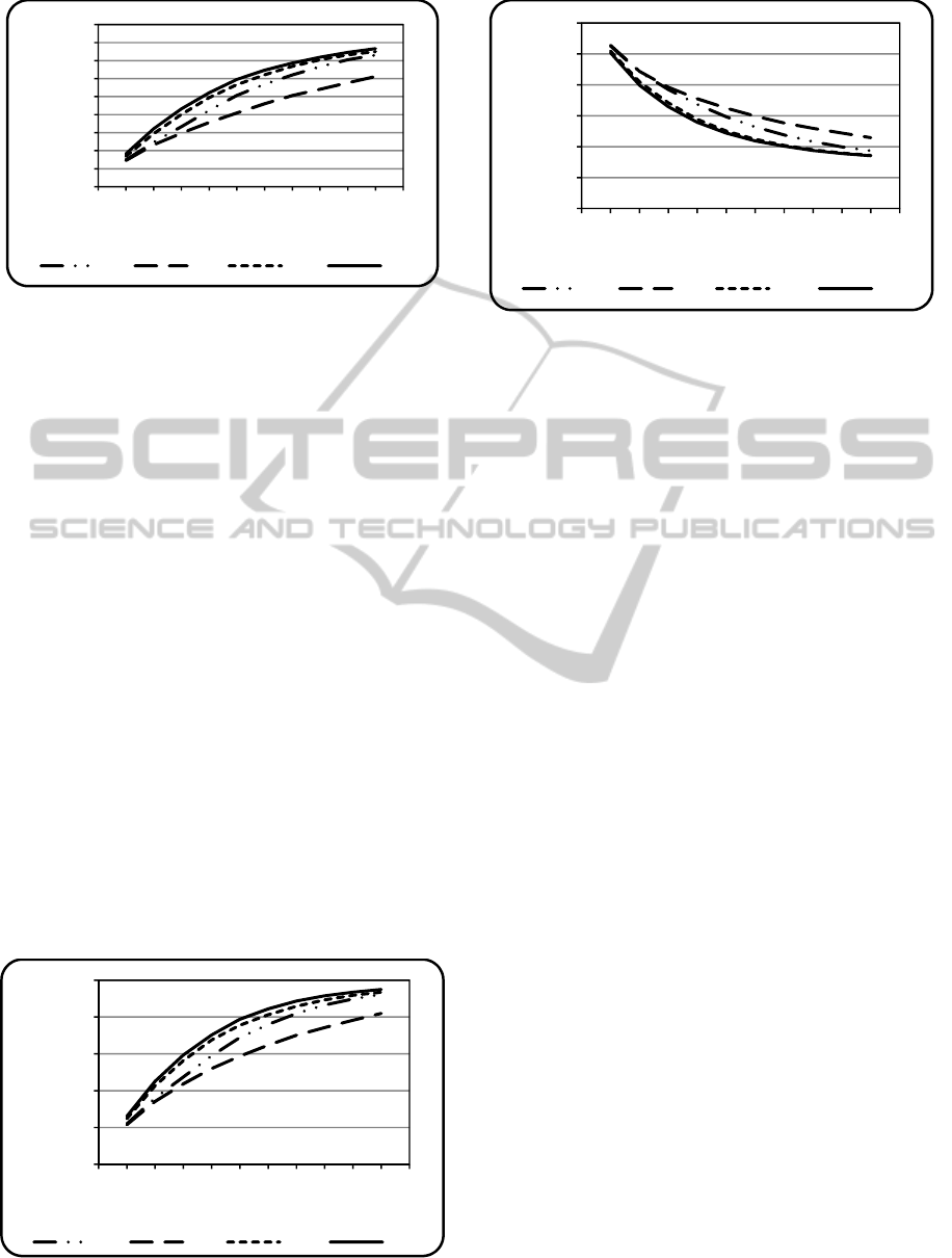
Figure 2: Percentage of correct predictions of CBRS,
CVRS, DWRS, and FWRS.
The PCP (coverage) increases as N
increases for
all RS. This increasing saturates as
reaches 80.
CVRS performs the worst among all RS we have
examined. This is because CVRS relies directly on
the ratings themselves. Raw ratings depend on each
user rating scale and on his mode and taste. Thus
comparing one user’s raw rating with another user’s
raw ratings will not give a good indication of their
similarity. This problem is alleviated with CBRS
and FWRS by using the deviation from each user’s
mean rating.
DWRS gives an indirect way for computing the
similarity between two users by summing the rating
difference weights not the differences themselves.
This approach performs better than both CBRS and
CVRS. However, it performs worse than FWRS
which employs both the deviation values and their
fuzzy weights. The MAE of FWRS is the minimum
amongst all the recommender systems we have
examined with all neighborhood set sizes. It starts to
saturate at N
90. MAE starts high because only a
few numbers of items can get predictions. Thus the
difference will be high, i.e. the actual ratings
themselves.
Figure 3: Coverage of CBRS, CVRS, DWRS, and FWRS.
Figure 4: Mean absolute error of CBRS, CVRS, DWRS,
and FWRS.
5 CONCLUSIONS
Pearson correlation coefficient is the most widely
used similarity measure for memory-based CRS.
However it is found that different users give
different weightings for their declared ratings. Thus
many methods have been proposed for introducing
weights to this similarity measure.
The proposed fuzzy weighting for Pearson
correlation coefficient is efficient in terms of time
and space. This fuzzy weighting is derived based on
the user rating deviation from his mean rating thus it
avoids the users’ different rating scales. Instead of
utilizing GA for small intervals which degrades the
usefulness of GA such that Bobadilla et al., (2011)
used, FWRS gives an easy way to get each user
fuzzy weights for different deviation values. This
weighting is not fixed and will change by changing
the neighbor. Experimental results show that FWRS
outperforms all the examined RSs in terms of PCP,
coverage, and mean absolute error.
This paper utilizes five fuzzy sets; however,
many ways can be proposed for fuzzifying the
deviation values. This is kept for future work.
REFERENCES
Goldberg, D., Nichols, D., Oki, B.M., and Terry, D., 1992.
‘Using collaborative filtering to weave an information
Tapestry’. Communication of the ACM, vol. 35 (12),
pp. 61-70.
Schafer, J. B., Frankowski, D., Herlocker, J., and Sen, S.,
2007. ‘Collaborative filtering recommender systems.
In the Adaptive Web’, LNCS 4321, P. Brusilovsky, A.
0
5
10
15
20
25
30
35
40
45
0 102030405060708090100110
PercentageofCorrectPredictions
(%)
NeighborhoodSetSize
CBRS CVRS DWRS FWRS
0
20
40
60
80
100
0 102030405060708090100110
Coverage(%)
NeighborhoodSetSize
CBRS CVRS DWRS FWRS
0
0,5
1
1,5
2
2,5
3
0 102030405060708090100110
MeanAbsoluteError
NeighborhoodSetSize
CBRS CVRS DWRS FWRS
Fuzzy-weightedPearsonCorrelationCoefficientforCollaborativeRecommenderSystems
413

Kobsa, and W. Nejdl. Eds., Berlin Heidelberg:
Springer-Verlag, pp. 291 – 324.
Burke, R., 2002. ‘Hybrid recommender systems: survey
and experiments’. User Modeling and User-Adapted
Interaction, vol. 12, pp. 331-370.
Adomavicius, G., and Tuzhilin, A., 2005. ‘Toward the
next generation of recommender systems: A survey of
the state-of-the-art and possible extensions’. IEEE
Trans. on Knowledge and Data Eng., vol. 17(6), pp.
734-749.
Al-Shamrri, Mohammad Yahya H., and Bharadwaj,
Kamal K., 2008. ‘Fuzzy-genetic approach to
recommender systems based on a novel hybrid user
model’. Expert Systems with Applications, Elsevier,
vol. 35(3), pp. 1386-1399.
Bobadilla, J., Ortega, F., Hernando, A., and Alcala, J.,
2011. ‘Improving collaborative filtering recommender
system results and performance using genetic
algorithms’. Knowledge Based Systems, Elsevier, vol.
24(8), pp. 1310-1316.
Min S-H., and Han, I., 2005. ‘Optimizing collaborative
filtering recommender systems’. In AWIC 2005, LNAI
3528, P.S. Szczepaniak and A. Niewiadomski. Eds.,
Berlin Heidelberg, Springer-Verlag, pp. 313–319.
Bharadwaj, Kamal K., and Al-Shamri, Mohammad Yahya
H., 2009. ‘Fuzzy computational models for trust and
reputation systems’. Electronic Commerce Research
and Applications, Elsevier, vol. 8, pp. 37-47.
Breese, J., Heckerman, D., and Kadie, C., 1998.
‘Empirical analysis of predictive algorithms for
collaborative filtering’. In Proceedings of the 14th
Conference on Uncertainty in Artificial Intelligence,
pp. 43-52, Madison, WI. Morgan Kaufmann, San
Francisco, CA.
Vozalis, E., and Margaritis, K., 2003. ‘Analysis of
recommender systems’ algorithms’. In Proceedings of
the sixth Hellenic-European Conference on Computer
Mathematics and its Applications (HERCMA), Athens,
Greece.
Han, J., and Kamber, M., 2006. Data Mining, Concepts
and Techniques. Morgan Kaufmann Publishers, 2
nd
edition.
Herlocker, J., Konstan, L., Terveen, L., and Riedl, J.,
2004. ‘Evaluating collaborative filtering recommender
systems’. ACM Transaction on Informartion Systems,
vol. 22(1), pp. 5-53.
ICEIS2013-15thInternationalConferenceonEnterpriseInformationSystems
414
