Parametric Fault Detection in Nonlinear Systems

A Recursive Subspace-based Approach

Paulo Gil

1,2

, F

abio Santos

, Alberto Cardoso

and Lu

ıs Palma

Departmento de Engenharia Electrot

ecnica, Faculdade de Ci

encias e Tecnologia

Universidade Nova de Lisboa, 2829-516 Caparica, Portugal

CISUC, Informatics Engineering Department, University of Coimbra, P

olo II, 3030-290 Coimbra, Portugal

Visteon Corporation Ltd, Electronics Product Group, 2951-503 Palmela, Portugal

Keywords:

Model-based Fault Detection, Parametric Faults, Subspace System Identiﬁcation, Recursive Parameters

Estimation, Neural Networks.

Abstract:

This paper deals with the problem of detecting nolinear systems’ parametric faults modeled as changes in

the eigenvalues of a local linear state-space model. The linear state-space model approximations are ob-

tained by recursive subspace system identiﬁcation techniques, from which the eigenvalues are extracted at

each sampling time. Residuals are generated by comparing the eigenvalues against those associated with a

local nominal model derived from a neural network predictor describing the nonlinear plant dynamics in free

fault conditions. Parametric fault symptoms are generated from the eigenvalues residuals, whenever a given

predeﬁned threshold is exceeded. The feasibility and effectiveness of the proposed framework is demonstrated

in a practical case study.

1 INTRODUCTION

Fault Detection and Isolation (FDI) consists of mak-

ing a binary decision concerning a malfunctioning hy-

pothesis, and in case of a given fault event to de-

termine its nature and location (Isermann and Ball

1997), (Isermann, 2011). In general, FDI frame-

works incorporate the concept of redundancy, ei-

ther in terms of hardware or analytical. While

the former approaches rely essentially on duplica-

tive signals provided by additional hardware, the an-

alytical or software redundancy uses a mathemati-

cal model of the plant along with dedicated esti-

mation methods (Hwang et al., 2010). Since this

methodology normally does not require additional

hardware it is usually more cost effective. How-

ever, this approach is more challenging owing to the

need of coping with model uncertainties, noise and

unknown/unmeasurable disturbances that ultimately

distorts the computed residuals and may lead to a mis-

classiﬁcation of symptoms.

Model-based fault detection and diagnosis meth-

ods use residuals between the plant and a mathemat-

ical model prediction in conjunction with a classiﬁer

or voter that, according to the residuals’ magnitude

and additional features, generates an alarm and pro-

vides information regarding the detected symptom.

Concerning residual generation methods, they can

be implemented based on state and output observers

(Chen and Patton, 1999), parity relations (Gertler,

1998) or on parameters estimation using system iden-

tiﬁcation techniques (Isermann, 1997), (Brito Palma

et al., 2005).

For a number of applications the FDI problem of

interest is to detect changes in the eigenstructure of

linear dynamic systems, being the structural vibration

monitoring a typical example. A straightforward ap-

proach relies on subspace-based linear system iden-

tiﬁcation (see e.g. (Moor et al., 1999)). In (Bas-

seville et al., 2000) subspace-based methods along

with the statistical local approach have been anal-

ysed in the context of designing fault detection al-

gorithms and suggested to be useful for in-operation

modal analysis and monitoring of mechanical struc-

tures subject to vibration, while in (Basseville et al.,

2007) it is presented an overview of theory and prac-

tice of covariance-driven input/output and output only

subspace-based algorithms for structural identiﬁca-

tion, damage detection and diagnosis, and sensor data

fusion.

In the preceding FDI works it is assumed that

the underlying system under monitoring is linear and

time-invariant. In the case of nonlinear systems these

methods are doomed to fail as a result of unreliable

Gil P., Santos F., Cardoso A. and Palma L..

Parametric Fault Detection in Nonlinear Systems - A Recursive Subspace-based Approach.

DOI: 10.5220/0004422100820088

In Proceedings of the 10th International Conference on Informatics in Control, Automation and Robotics (ICINCO-2013), pages 82-88

ISBN: 978-989-8565-70-9

 2013 SCITEPRESS (Science and Technology Publications, Lda.)

residuals due to the cumulative effect of model-plant

mismatch.

The main contribution of this work is to develop

a new framework to detect parametric faults in non-

linear dynamic systems, modelled as changes in the

internal system dynamics, by taking advantages of

recursive subspace-based system identiﬁcation tech-

niques, and the approximation capabilities of nonlin-

ear autoregressive with exogenous inputs Nonlinear

Autoregressive with Exogenous Inputs (NARX) neu-

ral networks. By assuming the input-output certainty

equivalence principle, the approach ﬁrst computes the

residuals of the underlying local eigenstructures. Sub-

sequently, by analysing these residuals, the change

detection module evaluates whether a parametric fault

has occurred.

2 SYSTEM IDENTIFICATION

In the context of fault detection and isolation a model

of the plant under normal or nominal operating condi-

tions is obtained by regression, upon selecting a par-

ticular model structure and a parametrization. When a

given fault affects the system it is most likely that the

system’s behaviour, in terms of outputs, inputs or in-

ternal dynamics, would differ from the behaviour pre-

dicted by the nominal operating model. This means

that fault events will be reﬂected in a change of the

models’ parameters. It is exactly this basic assump-

tion that most model-based identiﬁcation methods for

FDI consider in order to detecting and isolating faults

based on residual signals.

Among possible model structures to approximate

the input-output behaviour of the plant, the present

work considers linear state-space system models and

NARX neural networks, with the choice of these

model structures dictated by the nature of the pro-

posed FDI framework. In the case of linear state-

space model-based identiﬁcation the underlying ma-

trices are estimated by considering recursive subspace

techniques, while for NARX neural network predic-

tors their training is carried out ofﬂine using an itera-

tive optimization procedure.

2.1 Recursive Subspace Identiﬁcation

2.1.1 Preliminaries

In the case of ofﬂine SID methods it is implicitly as-

sumed that a sequence of input-output data collected

from the plant is available, that is,

{

u(0), u(1), . . . , u(N −1)

}

{

y(1), y(2), . . . , y(N)

}

(1)

In order to come up with estimates for the state-space

matrices (A, B,C, D) (up to within a similarity trans-

formation (Merc

ere, 2005)) and error covariance ma-

trices (Q, R, S) the estimation data are organized un-

der the form of past and future block Hankel matrices.

In what the input sequence is concerned, these block

Hankel matrices take the following form:







u(0) u(1) ··· u ( j −1)

u(1) u(2) ··· u( j)

u(i −1) u(i) ··· u (i + j −2)







(2)







u(i) u(i + 1) ··· u(i + j −1)

u(i + 1) u(i + 2) ··· u(i + j)

u(2i −1) u(2i) ··· u (2i + j −2)







(3)

and the past and future output block Hankel matrices,

≡Y

0|i−1

and Y

≡Y

i|2i−1

given according to,







y(0) y(1) ··· y ( j −1)

y(1) y(2) ··· y( j)

y(i −1) y(i) ··· y (i + j −2)







(4)







y(i) y(i + 1) ··· y(i + j −1)

y(i + 1) y(i + 2) ··· y(i + j)

y(2i −1) y(2i) ··· y (2i + j −2)







(5)

The block Hankel matrices of the stochastic subsys-

tem, built in with the outputs y

(k), the process noise

ω(k) and the measurement noise υ(k) are deﬁned as

above, namely, (Y

, Y

), (M

, M

) and (N

, N

), re-

spectively.

The past and future state vector sequence, respec-

tively, X

and X

take the following form:



x (0), x(1) , ··· x( j −1)





x (i), x(i + 1) , ··· x (i + j −1)



(6)

while the Toeplitz matrices associated with the deter-

ministic and the stochastic subsystems are given by:







D 0 0 ··· 0

CB D 0 ··· 0

CAB CB D ··· 0

i−2

B CA

i−3

B CA

i−4

B ··· D







(7)

ParametricFaultDetectioninNonlinearSystems-ARecursiveSubspace-basedApproach







0 0 0 ··· 0

C 0 0 ··· 0

CA CB 0 ··· 0

i−2

i−3

i−4

··· 0







(8)

The extended observability matrix associated with the

deterministic system is given by:







i−1







(9)

The following input-output matrix equations play

a fundamental role in subspace identiﬁcation (Bart

De Moor, 1999):

= Γ

+ H

= Γ

+ H

= Γ

+ H

+ N

= Γ

+ H

+ N

(10)

2.1.2 Recursive Algorithm

The algorithm implemented in this work comprises

two main stages: i) Online updating of the observa-

tion vector, using the QR factorization, along with

Givens rotations (see e.g. (Oku and Kimura, 2002),

(Merc

ere et al., 2004)) , and ii) Recursive estimation

of the extended observability matrix, considering the

online updating of the propagator.

i) QR Factorization Updating

Consider the following decomposition:













0 0













(11)

with Ψ the instrumental variable comprising past in-

puts and outputs, such that lim

j→∞

= 0, Θ

+ N

and rank



XΨ



= n. In such conditions

the following expression holds:

lim

j→∞

√

= lim

j→∞

√

X (12)

The procedure for updating the QR factorization with

the next data pair {u(τ), y(τ)} is as follows:





√





0 0





(τ + 1)

ψ(τ + 1)

(τ + 1)









(τ) 0

0 1





(13)

with λ ∈ R

a forgetting factor considered to weight

past information.

Now, by applying two sequences of Givens rota-

tions in (13) the factor R in the QR decomposition

is converted into the following block lower triangular

matrix:





√





0 0





(τ + 1)

ψ(τ + 1)

(τ + 1)





rot

(τ + 1) ·rot

(τ + 1) =





(τ + 1) 0 0 0

(τ + 1)

√

λR

(τ) 0

ψ(τ + 1)

(τ + 1)

√

λR

(τ)

√

λR

(τ) ˇz(τ + 1)





rot

(τ + 1) =





(τ + 1) 0 0 0

(τ + 1) R

(τ + 1) 0 0

(τ + 1) R

(τ + 1)

√

λR

(τ)

ˇz

(τ + 1)





(14)

with

ψ and ˇz vectors obtained after applying the ﬁrst

Givens rotation, and accounting for the information

included in u

, while

ˇz is the vector obtained after the

second Givens rotation in order to include the infor-

mation embedded in

ψ.

Taking into account (12) it follows that,



ˇz

−

ˇz



= Γ

(15)

Equation (15) shows that (14) leads asymptotically to

a given covariance matrix R

, from which the sub-

space spanned by the columns of the extended observ-

ability can consistently be extracted. The procedure

of recursively updating this covariance matrix is pre-

sented in the following equation:

(k) = λ

(k −1) + ˇz

(k) ˇz

(k) −

ˇz

(k)

ˇz

(k)

(16)

ii) Extended observability subspace basis updating

The process followed in this work for updating a

given basis for the extended observability matrix re-

lies on the propagator method (Munier and Delisle,

1991). This method has the advantage of enabling its

use in the context of coloured unknown disturbances.

Assume that the pair (A,C) is observable and the

system’s order n is known in advanced. Then, it is

possible to derive a given permutation matrix S ∈

li×li

such that the extended observability Γ

can be

decomposed in two blocks:

SΓ



∈ R

n×n

∈ R

(li−n)×n



(17)

Taking into account the propagator operator, (17) can

rewritten as,

SΓ





(18)

ICINCO2013-10thInternationalConferenceonInformaticsinControl,AutomationandRobotics

Now, by replacing (18) into (15) it follows that





¯x





(19)

which can be rewitten as,

ˇz

−R

ˇz

−R

ˇz

−R

ˇz

−R

ˇz



¯x



(20)

Equation (20) shows that the propagator can be found

by minimizing the following Frobenius norm:

J (P

) =



ˇz

−

ˇz

−P



ˇz

−

ˇz





(21)

In the case of all the involved matrices are nonsin-

gular (see (Merc

ere and Lovera, 2007)) the argument

of minimizing Eq. (21) is given by (Merc

ere et al.,

2008):



ˇz

−

ˇz



ˇz

−

ˇz



−1

(22)

This optimal solution can be recursively updated by

means of a Recursive Least Squares (RLS) algorithm.

iii) Estimation of State-space Matrices

Since recursive subspace identiﬁcation methods as-

sume that the vectorial basis dimension is known in

advanced the computation of estimates for the state-

space matrices is readily obtained from the extended

observability matrix and input-output data. For matri-

ces A and C the corresponding estimates are obtained

as follows:

C =

(1 : l, :)

A =



(1 : l (i −1) , :)



†

(l + 1 : li, :)

(23)

with





Concerning B and D estimates, they are found by

means of a least squares estimator applied to the ele-

ments of ζ(B, D) deﬁned as (dos Santos and de Car-

valho, 2003):

ζ(B, D) =



†

i−1

D 0



−





†

(24)

2.2 Neural Network Predictor

Multilayer perceptrons comprising one hidden layer

are universal approximators, that is, they are able to

approximate any nonlinear function with any desired

accuracy provided that some particular conditions are

held (see e.g. (Leshno et al., 1993), (Chen et al.,

1995)).

An important subclass of multilayer perceptrons,

quite appealing in the context of nonlinear control and

identiﬁcation, is the NARX neural networks, whose

input vector consists of past inputs and past outputs

(the regressor). This architecture can be analytically

represented as follows:

net

(k) = g (ϕ(k), θ)

(25)

with θ the neural network parameters vector consist-

ing of weights and biases, and the regressor ϕ (k)

given by:

(k) =(y (k −1), . . . , y(k −n

u(k −1) , . . . , u (k −n

))

(26)

where u(k) and y(k) denoting the system’s input and

output, n

and n

the lag windows for past inputs and

outputs, and g(·) a nonlinear mapping performed by

the NARX neural network. This input-output rela-

tionship can be rewritten as follows:

Regarding the activation functions of neurons in-

cluded in the output layer, they are all linear, while the

nonlinear activation functions σ(·) associated with

hidden layer neurons are chosen as continuous and

differentiable sigmoidal functions, upper and lower

bounded, satisfying the following conditions (Dong

et al., 2002):

• lim

t→±∞

σ(t) = ±1;

• σ(t) = 0 ⇐t = 0;

• σ

(t) > 0;

• lim

t→±∞

(t) = 0;

• max



(t)



≤ 1 ⇐ t = 0.

For the number of neurons to be incorporated

within each layer, only those associated with the out-

put layer are directly related to the number of out-

puts of the system. Concerning the hidden and input

layers, the number of neurons should be carefully se-

lected in order to enable the neural predictor to gen-

eralize well to unseen data, while presenting the min-

imal structural complexity. As such, there is a trade-

off between structural complexity and generalization

capability.

In the case of a three-layer NARX(N

, N

)

neural network, where N

, N

and N

, are respec-

tively, the number of input layer, hidden layer and out-

put layer neurons, with sigmoid activation functions

in the hidden layer and linear activation functions in

ParametricFaultDetectioninNonlinearSystems-ARecursiveSubspace-basedApproach

the remaining two layers, the corresponding output is

given by,

net

(k) = W

σ(W

·ϕ(k) + b

) + b

(27)

with W

∈ R

×N

, W

∈ R

×N

, b

∈ R

, b

∈ R

and the regressor vector given by (26).

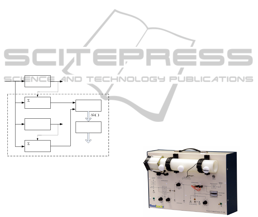
3 ARCHITECTURE

The framework for detecting parametric faults in non-

linear dynamic systems is based on comparing the

eigenstructure of two linear state-space realizations,

one for the nonlinear system under monitoring and

the other for the NARX neural network predictor. The

neural predictor was previously trained ofﬂine with an

informative enough dataset collected from the nonlin-

ear system in a fault-free context.

Process

(A,B,C,D)

Estimator

Neural

Network

(A,B,C,D)

Estimator

(k)

Residual

Generation

Decision

Making

Fault

Fault Detection

u(k)

y(k)

net

(k)

Figure 1: Parametric fault detection architecture.

Basically, the architecture (see Fig. 1) consists

of a linear state-space identiﬁcation module that es-

timates, through recursive subspace system identiﬁ-

cation techniques, local linear system matrices asso-

ciated with both the plant and the NARX neural net-

work predictor. Additionally, the platform includes

a residual generator module that computes, at each

discrete time k, and based on the eigenvalues of the

system matrices A

(k) and A

(k) a residual vector

∆λ(k) given by:

∆λ(k) =

(k) −λ

(k)

(28)

with

the element-wise absolute value operator.

The residuals ∆λ (k) are subsequently analysed in

the decision making module, which uses statistical

tools in order to test whether they have “signiﬁcantly”

deviated from zero. In particular, the decision crite-

rion is based on a threshold computed ofﬂine based on

the three-sigma limits approach (Montgomery, 2001).

If a residual exceeds the computed threshold the sys-

tem is considered in faulty operation and some ef-

fective measures should be taken to accommodate its

effects. Finally, it should be mentioned that fault

accommodation techniques are not the focus of this

work.

4 CASE STUDY

In this section the proposed approach for detecting

parametric faults in nonlinear dynamic systems is ex-

perimentally tested and validated using a laboratory

test-bed.

4.1 Test-bed

The test-bed consists of a heating system from

Feedback



, namely, the Process Trainer PCT 37-100

(Fig. 2). It comprises a variable-speed axial fan ad-

justed manually via a potentiometer, which circulates

an air-stream along a polypropylene tube. The airﬂow

rate is heated by means of a heating element under the

form of a grid with a maximum power of 80 W for an

input voltage of +10 V controlled by a thyristor cir-

cuit. A thermistor detector is included in the set-up

for sensing the temperature at one of the three avail-

able measurement points along the tube length.

The Process Control Trainer comprises a

heating element controlled by a thyristor

circuit which feeds heat into an airstream

circulated by an axial fan along a

polypropylene tube. A thermistor detector,

which may be placed at one of three

points along the tube length, senses the

temperature at that point.

The volume of air flow is controlled by

varying the speed of the fan.

Features

• A practical process in miniature

• Closed and open-loop continu-

ous control as well as two-step

control

• Fast response times

• Thermal time constants and time

transport lag

• Easy-to-read metering

Subject Areas

• Distance/Velocity Lag

• Transfer Lag

• Calibration

• Two-step Control

• Proportional Control System

Response

• Frequency Response

A comparison of these signals generates

a deviation signal which is applied to

the heater control circuit such that the

controlled condition is maintained at the

desired value. Two step (ON/OFF) and

Proportional band control is standard.

A change in setting represents a

supply side disturbance and the

effects are easily demonstrated.

The detector output is amplified to

provide both an indication of the

measured temperature and a feedback

signal for comparison with a set value

derived from a separate control.

Process

Control

37-100 SYSTEM

Process Control Trainer

Figure 2: Feedback



Process Trainer PCT 37-100.

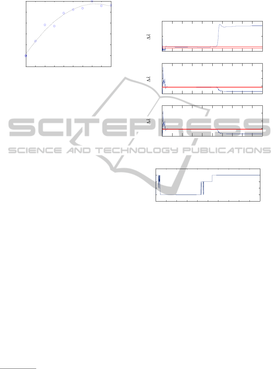
This setup represents a nonlinear time-varying

system, where the main source of nonlinearities are

associated with the input dependent static gain, while

the time variant behavior is essentially due to thermal

energy storage in the course of experiments. As can

be observed in Fig. 3, which shows the normalized

static gain as a function of the normalized input fed

to the system, the systems static gain varies with the

operation regime.

ICINCO2013-10thInternationalConferenceonInformaticsinControl,AutomationandRobotics

0.1 0.2 0.3 0.4 0.5 0.6 0.7 0.8 0.9 1

0.7

0.8

0.9

Normalized input

Normalized static gain

Figure 3: Feedback



Process Trainer PCT 37-100 static

gain.

The communication infrastructure between the

digital computer, where the fault detection platform

is installed, and the process trainer PCT 37-100 con-

sists of a peer-to-peer interconnection based on a data

acquisition board PMD-1208LS series, from the Mea-

surement Computing



. This device includes two 10-

bit analog outputs, 8 single-ended or 4 differential

analog inputs, and 16 digital I/O

4.2 Experiment

The experiment shown here was carried out consid-

ering the following nominal conﬁguration: fan speed

referred to the potentiometer’s position 5, tempera-

ture sensor located at position II (140 mm from the

heater grid), and a sampling interval of 10 ms. Re-

garding the linear state-space models’ complexity,

for Σ

= (A

, B

, D

) and Σ

= (A

, B

, D

they were both chosen to be of 3

order, as sug-

gested by the ofﬂine subspace algorithm. Regarding

the three-layered NARX neural network consisted of

four neurons in the input layer, seven neurons in the

hidden layer and one neuron in the output layer, while

the input to the network u

net

was represented by an ar-

ray of four elements, namely:

net

(k) = [u (k −1) u (k −2) y (k −1) y (k −2)]

(29)

In the experiment run the system’s fan potentiometer

was initially at position 5 and, subsequently, at sam-

ple 420, the fan speed was manually changed to 1.

This change resulted in a major air ﬂow rate reduc-

tion, which impacted the static gain and pure delay

of the system. Fig. 4 shows the three residuals over

time, computed from the eigenvalues of Σ

and Σ

and the experimental threshold associated with each

residual, while in Fig. 5 it is presented the number

see http://www.mccdaq.com.

of symptoms (out of three) corresponding to residuals

outside the thresholds.

0 100 200 300 400 500 600 700 800 9001000

0.05

0.1

0.2

0.3

0.4

0.1

0.2

0.3

0.4

Sample

0 100 200 300 400 500 600 700 800 9001000

Sample

123

Figure 4: Parametric fault - residuals and thresholds.

Symptoms

Sample

0 100 200 300 400 500 600 700 800 900 1000

Figure 5: Parametric fault - symptoms.

As can be observed in Fig. 5 at the beginning of

the experiment run, even still with no fault injected

on the system, the fault detection platform generates

unexpected symptoms. This behaviour is due to the

initialization of the subspace recursive estimation al-

gorithm, which in the initial phase is responsible for

residuals outside experimental thresholds. After this

initial time frame, the number of symptoms stabilizes

at zero, which is in line with the presence of no para-

metric fault acting on the system. With the fault in-

jected at sample 420 the system dynamics underwent

a noticeable change, which should be reﬂected in the

linear adaptive model of the process, and ultimately

be expressed by residuals lying outside the thresholds.

5 CONCLUSIONS

This paper addressed the problem of nonlinear para-

metric fault detection in nonlinear dynamic systems.

ParametricFaultDetectioninNonlinearSystems-ARecursiveSubspace-basedApproach

The proposed framework is based on recursive sub-

space system identiﬁcation techniques to generate

fault dependent symptoms from eigenvalues residu-

als. The parametric fault detection architecture was

tested on a nonlinear plant whose results demonstrate

the feasibility of the proposed approach in detecting

parametric faults.

ACKNOWLEDGEMENTS

This work has been supported by iCIS-Intelligent

Computing in the Internet of Services, Project

CENTRO-07-ST24-FEDER-002003.

REFERENCES

Bart De Moor, Peter Van Overschee, W. F. (1999). Algo-

rithms for subspace state space system identiﬁcation

- an overview. In Datta, B. N., editor, Applied and

Computational Control, Signals and Circuits: Volume

1: Vol 1, volume Vol. 1. Birkhauser.

Basseville, M., Abdelghani, M., and Benveniste, A. (2000).

Subspace-based fault detection algorithms for vibra-

tion monitoring. Automatica, 36(1):101 – 109.

Basseville, M., Benveniste, A., Goursat, M., and Mevel,

L. (2007). Subspace-based algorithms for struc-

tural identiﬁcation, damage detection, and sensor

data fusion. EURASIP J. Appl. Signal Process.,

2007(1):200–200.

Brito Palma, L., Coito, F., and Neves da Silva, R. (2005).

Diagnosis of parametric faults based on identiﬁcation

and statistical methods. In Decision and Control, 2005

and 2005 European Control Conference. CDC-ECC

’05. 44th IEEE Conference on, pages 3838 – 3843.

Chen, J. and Patton, R. (1999). Robust Model-Based Fault

Diagnosis for Dynamic Systems. Kluwer Academic

Publishers.

Chen, T., Chen, H., and wen Liu, R. (1995). Approxi-

mation capability in c(r macr;n) by multilayer feed-

forward networks and related problems. Neural Net-

works, IEEE Transactions on, 6(1):25 –30.

Dong, Q., Matsui, K., and Huang, X. (2002). Existence and

stability of periodic solutions for hopﬁeld neural net-

work equations with periodic input. Nonlinear Analy-

sis: Theory, Methods & Applications, 49(4):471 479.

dos Santos, P. and de Carvalho, J. (2003). Improving the

numerical efﬁciency of the b and d estimates pro-

duced by the combined deterministic-stochastic sub-

space identiﬁcation algorithms. In Decision and Con-

trol, 2003. Proceedings. 42nd IEEE Conference on,

volume 4, pages 3473 – 3478 vol.4.

Gertler, J. (1998). Fault Detection and Diagnosis in Engi-

neering Systems. Marcel Dekker.

Hwang, I., Kim, S., Kim, Y., and Seah, C. (2010). A survey

of fault detection, isolation, and reconﬁguration meth-

ods. Control Systems Technology, IEEE Transactions

on, 18(3):636 –653.

Isermann, R. (1997). Supervision, fault-detection and fault-

diagnosis methods: An introduction. Control Engi-

neering Practice, 5(5):639 – 652.

Isermann, R. (2011). Fault-Diagnosis Applications.

Springer-Verlag.

Isermann, R. and Ball

e, P. (1997). Trends in the applica-

tion of model-based fault detection and diagnosis of

technical processes. Control Engineering Practice,

5(5):709 – 719.

Leshno, M., Lin, V. Y., Pinkus, A., and Schocken, S. (1993).

Multilayer feedforward networks with a nonpolyno-

mial activation function can approximate any func-

tion. Neural Networks, 6(6):861 – 867.

Merc

ere, G. (2005). Contribution

a l’identiﬁcation

ecursive des syst

emes par l’approche des sous-

espaces (in French). PhD thesis, Universit

e des Sci-

ences et Technologie de Lille, France.

Merc

ere, G., Bako, L., and Lecœuche, S. (2008).

Propagator-based methods for recursive subspace

model identiﬁcation. Signal Processing, 88(3):468–

491.

Merc

ere, G., Lecœuche, S., and Lovera, M. (2004). Re-

cursive subspace identiﬁcation based on instrumental

variable unconstrained quadratic optimization. Inter-

national Journal of Adaptive Control and Signal Pro-

cessing, 18(9-10):771–797.

Merc

ere, G. and Lovera, M. (2007). Convergence analysis

of instrumental variable recursive subspace identiﬁca-

tion algorithms. Automatica, 43(8):1377 – 1386.

Montgomery, D. C. (2001). Introduction to Statistical Qual-

ity. John Wiley & Sons.

Moor, B. D., Overschee, P., and Favoreel, W. (1999). Al-

gorithms for subspace state-space identiﬁcation: An

overview. In Datta, B. N., editor, Applied and compu-

tational control, signals, and circuits, volume 1, chap-

ter 6, pages 247 – 311. Birkhuser.

Munier, J. and Delisle, G. (1991). Spatial analysis using

new properties of the cross-spectral matrix. Signal

Processing, IEEE Transactions on, 39(3):746 –749.

Oku, H. and Kimura, H. (2002). Recursive 4sid algorithms

using gradient type subspace tracking. Automatica,

38(6):1035 – 1043.

ICINCO2013-10thInternationalConferenceonInformaticsinControl,AutomationandRobotics