Static Output-feedback Control with Selective Pole Constraints
Application to Control of Flexible Aircrafts
Isaac Yaesh
1
and Uri Shaked
2
1
IMI, Advanced Systems Division, Ramat Hasharon 47100, Israel
2
School of Electrical Engineering, Tel-Aviv University, Tel-Aviv 69978, Israel
Keywords:
H
∞
-optimization, Flight Control, Flexible Aircraft, Pole Placement.
Abstract:
A non-smooth optimization approach is considered for designing constant output-feedback controllers for
linear time-invariant systems with lightly damped poles. The design requirements combine H
∞
performance
requirements with regional pole constraints excluding high frequency lightly damped poles. In contrast to the
usual (full) pole-placement (FPP) problem, the problem dealt here is one of Selective Pole Placement (SPP).
The latter design problem is frequently encountered in the control of aircraft with non-negligible aeroelastic
modes which are too fast to be handled by the control surface actuators. As in the FPP case, the pole constraints
are embedded in the design criterion using a transformation on the system model which modifies the H
∞
-norm
of the closed-loop system via a barrier function that is related to the closed-loop poles damping. Dissimilar to
the closed-loop solution that is designed for the FPP, in the SPP case, numerical calculations of the gradient of
the cost function is needed. The proposed method is applied to a flight control example of a flexible aircraft.
1 INTRODUCTION
The static output-feedback control problem has at-
tracted the attention of many in the past (Bernstein
et al., 1989)-(Yaesh and Shaked, 1997). The main
advantage of static output-feedback is the simplicity
of its implementation and the ability it provides for
designing controllers of prescribed structure such as
PI and PID. As in other control related fields, PI and
PID controllers are widely applied in the aerospace
industry. When aircraft or missiles possess flexible
modes which are within or close to the desired use-
ful system bandwidth, one may either try to damp the
dynamic modes or just try to provide the control sys-
tem means to avoid excitation of these modes. The
latter is the common case, and it is widely encoun-
tered in practice due to bandwidth and slew rate lim-
itations of the control surface actuators (e.g. electri-
cal or hydraulic servo systems) and due to possibly
large uncertainties in the parameters (i.e. natural fre-
quency and damping) which characterize the flexible
modes. The uncertainty in the natural frequency is the
result of modelling errors, which in turn are caused
by data inaccuracy of the mass distribution model.
Since the damping may possess a nonlinear behav-
ior (e.g. large damping for large input amplitudes
and small one for small amplitudes), one has to take
into account the whole range of damping coefficients.
One may conclude in such cases that the controller
should minimize a performance criterion subject to
pole-placement constraints (e.g. damping coefficient)
of the rigid modes poles. The rigid pole modes for
which pole-placement requirements are applied can
be differed from the flexible modes poles, by their nat-
ural frequency. Namely, poles which possess a natural
frequency above some pre specified bound are classi-
fied as belonging to flexible modes and are not to be
re-placed. Noting that performance (e.g. bandwidth)
requirements as well as robust stability requirements
(e.g. gain and phase margin) can be achieved using
H
∞
-norm minimization, one may apply one of the
available tools that enable the design of static output-
feedback controllers ((Burke et al., 2006),(Apkarian
and Noll, 2006)). In such designs, the closed-loop
damping of the dominant poles can not be guaranteed
and, therefore, one may end up with an under damped
closed-loop.
In (Yaesh and Shaked, 2012) the H
∞
-optimization
problem with pole-placement constraints has been
solved by adopting the non-smooth optimization ap-
proach of (Burke et al., 2006) to deal with pole con-
straints. There, the pole-placement requirement has
been used to modify the H
∞
-norm cost function using
a barrier function (i.e. large penalty when constraints
153
Yaesh I. and Shaked U..
Static Output-feedback Control with Selective Pole Constraints - Application to Control of Flexible Aircrafts.
DOI: 10.5220/0004439201530160
In Proceedings of the 10th International Conference on Informatics in Control, Automation and Robotics (ICINCO-2013), pages 153-160
ISBN: 978-989-8565-70-9
Copyright
c
 2013 SCITEPRESS (Science and Technology Publications, Lda.)

are violated) and the gradient of this barrier function
has been evaluated in closed-form, allowing efficient
use of (Burke et al., 2006). In the present paper, the
application of the pole-placement requirements is re-
stricted only to the poles which are classified as the
rigid modes of the plant whereas the flexible modes
remain untouched as much as possible. The design
for this selective requirement on the poles is the sub-
ject of the present paper.
Since the chosen H
∞
-optimization method for
static output-feedback design is the one of (Burke
et al., 2006) some short (and not complete) survey of
other methods may be in place. In this context, one
should mention that the static output-feedback syn-
thesis problem is known to be non-convex, and that
many algorithms have been presented that combine
convex methods with iterative solutions. One can
mention, at this context, the algorithm in (Iwasaki,
1999) which, under some assumptions, is found to
converge in stationary infinite horizon examples with-
out uncertainty. The static output-feedback synthe-
sis problem is characterized in (Iwasaki, 1999) by in-
equalities which are bilinear in the variable matrices.
Therefore, standard convex programming procedures
could not be used in the past to solve the problem,
even in the case where the system parameters were all
known, and various methods were proposed to deal
with this difficulty (see e.g. (Peres et al., 1999) and
(Leibfritz, 2001)). Another approach is the one of di-
rect search which has been explored in (Simon, 2011)
and (Esquivel et al., 2011). Recently, a non-smooth
optimization approach to H
∞
-optimization has been
suggested in (Apkarian and Noll, 2006) and (Burke
et al., 2006). These methods utilize recently de-
veloped quadratic programming techniques for non-
smooth functions.
The method of the present paper is successfully
applied to the control problem of a flexible aircraft
where the rigid mode control is designed to avoid both
modification and excitation of the flexible modes.
Notation: Throughout the paper the superscript
‘T’ stands for matrix transposition, R
n
denotes the n
dimensional Euclidean space and R
n×m
is the set of
all n × m real matrices. For a symmetric P ∈ R
n×n
,
P > 0 means that it is positive definite. The no-
tation col{a, b} for vectors a and b represents the
augmented vector [a
T
b
T
]
T
. For square A ∈ R
n×n
,
λ(A) denotes its eigenvalues whereas α(A) denotes
its spectral abscissa(Apkarian and Noll, 2006). For
two matrices A and B of the appropriate dimensions
we denote the matrix product in the usual sense by
AB and their Kronecker product by A
N
B. We also
denote by Tr{A} the trace of a matrix A. For a com-
plex scalar z = x + iy where i
2
= −1. Also note that
the integer i = 1,2,... is also used as index. Distin-
guishing between these two uses will be by the con-
text. We also denote ¯z = x − iy which is not to be
confused by e.g.
¯
A which is just a notation of a real-
valued matrix. In this paper we provide all spaces
R
k
, k ≥ 1 with the usual inner product < ·,· > and
with the standard Euclidean norm || · ||. We denote
by L
2
the space of square-integrable functions. For
a transfer-function matrix G(s) =
¯
C(sI −
¯
A)
−1
¯
B +
¯
D
where
¯
A is Hurwitz, we denote by ||G||
∞
its H
∞
-
norm. Note that ||G||
∞
< γ with w and z being, re-
spectively, the input and output signals of G, cor-
responds both to ||z||
2
2
− γ
2
||w||
2
2
< 0 for all w ∈ L
2
and sup
Ω∈R
¯
σ[G(iΩ]) where
¯
σ denotes the maximum
singular value. The gradient with respect to a ma-
trix X ∈ R
n×m
of a scalar function f (x) is defined
by
∂f(X)
∂X
:= {G
ij
} where G
ij
= lim
δ→0
f(X+e
i
e
T
j
δ)− f (X)
δ
where e
i
is the i’th unit column vector. The di-
rectional derivative of f(X) along the direction Y ∈
R
n×m
which is defined by lim
δ→0
f(X+Yδ)− f (X)
δ
=
Tr{Y
T
∂f(X)
∂X
}. Also note that in case of f(X) −
f(X + ∆) = Tr{S∆} + o(∆), it is readily obtained
that [
∂f(X)
∂X
]
ij
= lim
δ→0
Tr{Se
i
e
T
j
δ}+o(δ)
δ
= S
ji
. Namely,
∂f(X)
∂X
= S
T
. We finally note that in order to avoid
confusion, the output vector of the linear system is
denoted by the boldface z while a complex scalar is
denoted just by z.
2 PROBLEM FORMULATION
We consider the following linear system
˙x = Ax(t) + B
1
w(t) + B
2
u(t), x(0) = x
0
y = C
2
x(t)
(1)
with
z(t) = C
1
x(t) + D
12
u(t) (2)
where x ∈ R
n
is the system state vector, w ∈ R
q
is the exogenous disturbance signal, u ∈ R
ℓ
is the
control input, y ∈ R
m
is the measured output and
z ∈ R
r
⊂ R
n
is the state combination (objective func-
tion signal) to be regulated. The matrices A,B
1
,C
1
,C
2
and D
12
are constant matrices of appropriate dimen-
sions.
We seek a controller
u = Ky, (3)
where K is a constant gain matrix, that achieves a
certain performance requirement. The design of K
should comply with the following requirements:
• The H
∞
-performance requirement: Assuming
that the exogenous disturbance signal is energy
bounded (i.e. w ∈ L
2
), a prescribed disturbance
ICINCO2013-10thInternationalConferenceonInformaticsinControl,AutomationandRobotics
154

attenuation factor γ should be guaranteed, so that
J
∞
< 0 where
J
∞
:= ||z(t)||
2
2
− γ
2
||w(t)||
2
2
(4)
• The closed-loop poles damping ratio con-
straint: To define this design constraint one first
defines the maximum natural frequency ω
R
(the
subscript R stands for ”rigid”) so that when a pole
s∈ C satisfies |s| < ω
R
, it is classified to be a mode
of the rigid body dynamics. Then pole-placement
requirement is defined to ensure that the eigen-
values λ
j
= r
j
e
iθ
j
, j = 1,2,..n with natural fre-
quency smaller than ω
R
of A+B
2
KC
2
should pos-
sess large enough damping ratios:
min
r
j
≤ω
R
,, j=1,2,...,n
{ζ
j
} ≥ ζ
min
(5)
where ζ
j
:= cos(θ
j
).
3 PROBLEM SOLUTION
The requirements of the previous section are on the
closed-loop system which is obtained by substituting
(3) into (1). The closed-loop system is
˙x = (A+ B
2
KC
2
)x(t) + B
1
w(t) :=
¯
Ax+
¯
Bw, x(0) = x
0
z = (C
1
+ D
12
KC
2
)x(t) :=
¯
Cx
(6)
To solve the above problem of combined H
∞
-
performance and closed-loop damping requirement
we should first put the latter in a tractable form. De-
noting, to this end, cos(θ) = ζ
min
, the latter pole-
placement requirement is equivalent ((Chilali and
Gahinet, 1996) ) to f
D
(z) < 0 where
f
D
(z)=

sin(θ)(z+¯z) −cos(θ)(z−¯z)
cos(θ)(z−¯z) sin(θ)(z+ ¯z)

=W
T
z+W¯z
(7)
and where
W =

sin(θ) cos(θ)
−cos(θ) sin(θ)

(8)
We next invoke the result of (Arzelier et al., 1993)
which states, for our case, that (7) is satisfied if and
only if there exists P > 0 so that
(W
O
¯
A)P+ P(W
O
¯
A)
T
< 0 (9)
Moreover, it was shown in (Chilali and Gahinet,
1996) that the structure of P is block diagonal with
equal blocks, namely that the existence of P > 0
which satisfies (9) is equivalent to the existence of
X > 0 so that
(W
O
¯
A)

X 0
0 X

+

X 0
0 X

(W
O
¯
A)
T
< 0
(10)
where
¯
A
W
=W
O
¯
A=

W
11
¯
A W
12
¯
A
W
21
¯
A W
22
¯
A

= (11)

sin(θ)
¯
A cos(θ)
¯
A
−cos(θ)
¯
A sin(θ)
¯
A

Writing (10) more explicitly, we obtain

(
¯
AX + X
¯
A
T
)sin(θ) (
¯
AX − X
¯
A
T
)cos(θ)
−(
¯
AX − X
¯
A
T
)cos(θ) (
¯
AX + X
¯
A
T
)sin(θ)

< 0
(12)
The latter inequality guarantees the damping require-
ment. We, therefore, resort to the recently suggested
approach of non-smooth optimization (NSO) ((Ap-
karian and Noll, 2006) and (Burke et al., 2006)) and
define, to this end, a cost function which combines the
H
∞
-performance criterion and the criterion of min-
imum closed-loop poles damping. The combined
cost function is just the H
∞
-norm of the closed-loop,
whenever the eigenvalues λ
j
= r
j
e
iθ
j
, j = 1, 2,..n of
¯
A satisfy either ζ
j
≥ ζ
min
, or r
j
> ω
R
. Whenever
ζ
j
< ζ
min
and r
j
≤ ω
R
the cost function is increased
monotonicallywith ζ
min
−ζ
j
, using a barrier function.
We note that one could suggest defining a subset
of C
R
∈ C where any re
iθ
∈ C
R
satisfies either r > r
R
or cos(θ) > ζ
min
and then finding a matrix W, replac-
ing the one of (8) by a new W
R
, so that (10) will be
satisfied by W
R
. If such W
R
could be found, one could
just apply the results of (Yaesh and Shaked, 2012) to
design static output-feedback controllers for flexible
aircrafts which satisfy the requirements of Section 2
above.
Unfortunately C
R
is not a convex set and, there-
fore, such W
R
does not exist. We, therefore, resort to
the analysis of the eigenvalues λ(
¯
A
W
) of
¯
A
W
. To this
end, we invokethe following property of the spectrum
of W
N
¯
A.
Lemma 1. Let λ
j
, j = 1,2,...,n and µ
1
,µ
2
be re-
spectively the eigenvalues of A and W. Then, the
eigenvalues ofW
N
¯
A are λ
i
µ
k
, j = 1,2,...,n, k = 1,2.
Since, however, W of (8) is an orthogonal matrix,
we have |µ
1
| = |µ
2
| = 1 leading to
|λ
j
(
¯
A
W
)| = |λ
j
(
¯
A)|
The eigenvalues of
¯
A which are with natural fre-
quencies smaller than or equal to ω
R
are, therefore,
mapped to eigenvalues of
¯
A
W
with the same property.
Consider the spectral abscissa (see e.g.
(Apkarian and Noll, 2006)) of
¯
A and define
its natural-frequency restricted version, by
α
R
(
¯
A) := max
j=1,2,...n
Real(λ
j
;|r
j
| < ω
R
) where
λ
j
= r
j
e
iθ
j
, j = 1,2,...n denote the eigenvalues of
¯
A.
The following result is then readily obtained from (9)
and Lemma 1:
Lemma 2. Consider the system ˙x =
¯
Ax. The in-
equality (5) is satisfied if and only if α
R
(
¯
A
W
) < 0.
We, therefore, consider the following cost func-
StaticOutput-feedbackControlwithSelectivePoleConstraints-ApplicationtoControlofFlexibleAircrafts
155

tion :
f(K)=||
¯
C(K)(sI−
¯
A(K))
−1
¯
B(K)||
∞
+ρβ(K)α
R
(
¯
A
W
(K))
(13)
where ρ >> 1 is a scalar, and
β(K) =

0 if α
R
(
¯
A
W
(K)) < 0
1 if α
R
(
¯
A
W
(K)) ≥ 0

We note that in the script files that accompany
(Burke et al., 2006), ||
¯
C(sI −
¯
A)
−1
¯
B||
∞
have been de-
fined, and both the value of f and its gradients with
respect to
¯
A,
¯
B,
¯
C and
¯
D are provided. Also there, the
function α(
¯
A) and its gradient with respect to
¯
A are
provided.
The first part in the cost function (13), namely the
H
∞
component, can therefore be computed by just us-
ing the above formulae for the H
∞
-norm and its gradi-
ent which are programmed in the script function hin-
fty.m in (Burke et al., 2006). The second part in the
cost function (13), which corresponds to the damp-
ing component via α
R
(
¯
A
W
(K)), is computed using
Lemma 1 above. Note that it requires the compu-
tation of all the eigenvalues of
¯
A. For the gradient
of the second component, we need to derive a for-
mula for ∂α
R
(
¯
A
W
(K))/∂
¯
A. We recall from (Yaesh
and Shaked, 2012) that for the case where ω
R
tends
to infinity (namely all the poles are classified as rigid
body poles) α
R
() is replaced by α() and one may de-
note H := ∂α(
¯
A
W
)/∂
¯
A and partition the gradient of
α(
¯
A
W
) with respect to
¯
A
W
conformally with the parti-
tion of
¯
A
W
in (11) as
∂α(
¯
A
W
)
∂
¯
A
W
=

G
11
G
12
G
21
G
22

(14)
and obtain that
H = G
11
W
11
+ G
12
W
12
+ G
21
W
21
+ G
22
W
22
However for finite ω
R
one needs an explicit (and un-
fortunately CPU consuming) numerical calculation of
H. Namely, use the definition,
H = {H
ij
},i = 1,2,...n, j = 1, 2,..., n (15)
where
H
ij
= ∂α
R
(W
O
¯
A)/∂
¯
A
ij
(16)
= lim
δ→0
[α
R
(W
O
(
¯
A+ e
i
e
T
j
δ)) − α
R
(W
O
¯
A)]/δ
and where e
i
∈ R
n
is the i’th unit column vector.
Since G of (14) can then be computed using the script
file specabsc.m in (Burke et al., 2006) we can com-
pute
f(
¯
A,
¯
B,
¯
C) = ||
¯
C(K)(sI −
¯
A)
−1
¯
B||
∞
+ ρβα(
¯
A
W
)
:= f
1
(
¯
A,
¯
B,
¯
C) + f
2
(
¯
A)
(17)
where f
1
(
¯
A,
¯
B,
¯
C) and f
2
(
¯
A) are respectively com-
puted using the script files hinfty.m and specabsc.m
in (Burke et al., 2006). As f
2
does not depend on
¯
B and
¯
C, the gradients of f with respect to
¯
B,
¯
C are
still computed using hinfty.m in (Burke et al., 2006)
whereas the gradient of f with respect to
¯
A is derived
using
∂f
∂
¯
A
=
∂f
1
∂
¯
A
+
∂f
2
∂
¯
A
where the second term is computed using (15) and
(16).
Remark 1: It may be seen at first sight, that the
above closed-loop damping requirements can be al-
ways satisfied. Obviously, such a conclusion is wrong
due to the following reasons:
• If the plant is uncontrollable, its uncontrollable
poles with natural frequency smaller than ω
R
,
must posses the minimum required damping ra-
tio.
• Even if the latter condition is satisfied, there is
no guarantee that static output-feedback suffices
to place the poles according to the requirements.
In such a case, one may apply either a full-state
feedback or under an appropriate observability as-
sumption, a full-order controller. Note that in
some cases, where static output-feedback does
not suffice, reduced-order controllers maybe ad-
equate.
Remark 2: The cost function of (13) together
with (4) involve a tradeoff between the disturbance
attenuation γ and the required damping coefficient
ζ
min
. Since for large enough ρ, the suggested solu-
tion scheme involves minimization of γ subject to the
damping coefficient constraint, one may explore the
tradeoff by varying ζ
min
.
4 FLEXIBLE AIR VEHICLE -
CONTROLLER DESIGN ON
NOTCH FILTERED PLANT
This example deals with a flexible air vehicle, where
the suggested controller includes a 6th order bending-
modes-filter (BMF) consisting of a cascade of 4th or-
der notch filter and a 2nd order low-pass filter, to at-
tenuate the effect of the bending modes, and a simple
PID (Proportional + Integral + Derivative) controller
which operates on the filtered plant outputs.
The PI controller gains are then tuned using the
method of the present paper, where the original plant
is replaced by the augmented plant which includes the
BMF in cascade.
ICINCO2013-10thInternationalConferenceonInformaticsinControl,AutomationandRobotics
156

The suggested method avoids tuning of a higher
order controller which would be of order 7 including
the BMF (order 6) and the tracking error integrator.
If such a 7th order controller were designed for dif-
ferent flight conditions, the resulting controller would
be expected to possess an intricate dependence on the
flight condition parameters (e.g. Mach number, dy-
namic pressure and so on). In the suggested control
method, the central frequency of the notch filter, sim-
ply depends on the 1st order flexible mode natural fre-
quency (which in turn depends on the fuel mass in the
vehicle, its take off configuration etc.). The tuned pa-
rameters are then the PID gains only, leaving 3 pa-
rameters only for gain scheduling.
We consider a single flight condition (Mach no.
0.62) of the vehicle where the airframe G
a
(s) =
C
a
(sI − A
a
)
−1
B
a
+ D
a
state-space representation is :
A
a
=






−0.2064 −702.6 0.01184 0 0
0.00737 −0.54 0 0 0
0 1.473 0 0 0
0 0 0 0 1
−3.93 0 0 −64337 −3.551






B
a
= col{8.0128, 17.66, 0,0, 2543.3}
C
a
=

0 1 0 0 0.037165
0 0 1 0.037165 0

and
D
a
= col{0,0}
The states in this representation are x =
col{v,r,ψ,q
1
,q
2
} where v is the lateral component of
the airspeed, r is the yaw-rate, ψ is the azimuth and
q
1
,q
2
are the states of the 1st order bending mode.
The input in this representation is the rudder angle δ
r
and the outputs are the versions ¯r and
¯
ψ of respec-
tively r and ψ which are affected by the flexible dy-
namics.
The servo model G
S
(s) which generates the rudder
angle δ
r
from the corresponding command u is de-
scribed by a second order system with unit DC gain,
a natural frequency of 113rad/sec and damping coef-
ficient of 0.7.
The BMF is givenby G
BMF
(s) =
1
(1+sτ)
2
G
2
Notch
(s):
G
Notch
(s) =
s
2
+ 2ζ
1
ωs+ ω
2
s
2
+ 2ζ
2
ωs+ ω
2
where ζ
1
= 0.005, ζ
1
= 0.2,ω = 2π × 40.4rad/sec
and τ =
1
2π×60
sec..
An integral weight on the azimuth angle error ψ−
ψ
c
is defined, as well as weights on the output ψ and
and the rudder command u. The minimized output is:
z = col{
5
s
(ψ− ψ
c
),ψ, 0.3u}
We define the exogenous disturbance to be w := ψ
c
.
We note that the first component in the transference
T
zw
relating w and z, corresponds to a weighted (via
5/s) version of the sensitivity S(s) = (1 + KP(s))
−1
.
The second term there correspondsto the complemen-
tary sensitivity T(s) = 1−S(s) whereas the third term
is just the control effort transference relating u and
w = ψ
c
.
The overall plant consists of the airframe G
a
(s)
cascaded with the BMF, the 2nd order model G
R
(s)
of the rate sensor (natural frequency of 90rad/sec
and damping coefficient of 0.125) and a pure delay
of 2.5msec represented by 2nd order Pade’ approxi-
mation G
D
(s). It is given by :
P(s) = G
R
(s)G
D
(s)G
S
(s)G
BMF
(s)G
a
(s)
The measured outputs vector is chosen as :
y = col

¯r,
¯
ψ,
5
s
(
¯
ψ− ψ
c
)}

A couple of the PID-like controller designs are
compared :
• H
∞
control without pole-placement (Burke et al.,
2006). The results of this attempt are illustrated
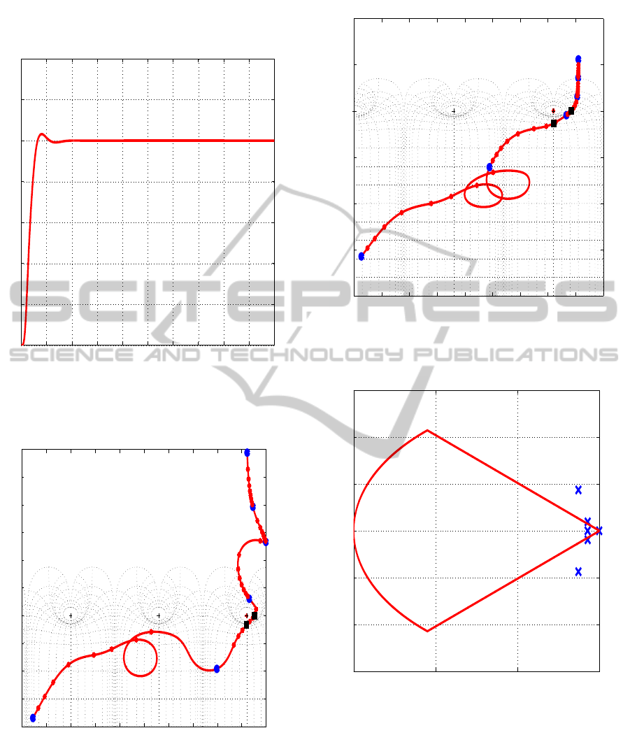
in Figures 1 - 4. We see in Fig. 1 a satisfying
step response, but somewhat low stability mar-
gins when loop is cut at control (about 7 db and
32 degrees phase margin (see Fig. 2). The stabil-
ity margins when loop is cut at the feedback (Fig.
3) are higher (about 13 db and 64 degrees phase
margin). Note that the low overshoot in the step
response to ψ
c
is associated with the high stability
margins when the loop is cut at the feedback. This
is since the transference from ψ
c
to ψ is L/(1+L)
where L is just the loop transfer function obtained
when cutting the loop in the feedback. The control
gains are K =

−1.1823 −11.802 −14.8

.
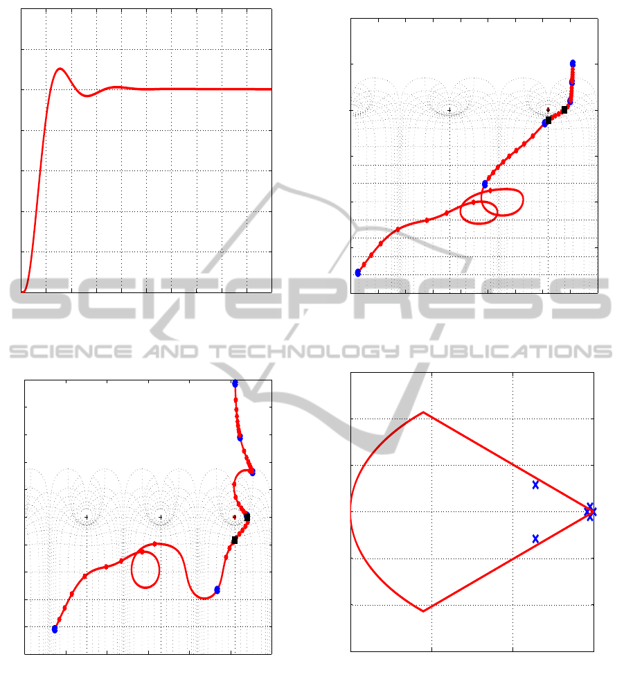
• H
∞
/ SPP control with an attempt to place only
the poles with natural frequency smaller than
ω
R
= 150rad/sec to have damping ratio of 0.4
or larger : With the method of the present paper,
all poles within 150rad/sec possess damping ra-
tios greater than or equal to 0.4. The closed-loop
poles complying with the design requirements are
shown in Fig. 8 (see also Fig. 4 to compare to
the case where no pole-placement requirements
are imposed). The closed-loop step response is
depicted in Fig. 5, whereas the corresponding
Nichols chart when loop is cut in the feedback is
depicted in Fig. 7. The somewhat larger over-
shoot in the step response is due to the lower mar-
gins at the feedback cut. However, when loop is
open at the control signal (see Fig. 6) one no-
tices that the gain and phase margin are much
improved (16db and 62 degrees) with respect to
StaticOutput-feedbackControlwithSelectivePoleConstraints-ApplicationtoControlofFlexibleAircrafts
157

the corresponding margins in design using the
original method of (Burke et al., 2006) without
pole placement requirements . Since larger un-
certainties are expected at the plant input (aero-
dynamic and flexible mode dynamics uncertain-
ties), where no significant uncertainties are ex-
pected in the feedback, one may conclude that
design with the H
∞
/ SPP method of the present
paper, has improved robust stability with respect
the design with (Burke et al., 2006) with no mod-
ifications. The improved stability margins are
achieved at the cost of some degradation in the
step response to command. One should, how-
ever, keep in mind that the command response
can be readily improved with a shaping filter (i.e.
2 degrees of freedom compensator) without any
cost regarding stability. The control gains are
K =

−0.47704 −2.0889 −1.4118

.
Remark 3: As noted above, the notch filter G
Notch
attenuates the 1st order flexible mode (which is
included in the plant model G
a
(s)) whereas the
second order low-pass filter
1
(1+sτ)
2
in G
BMF
(s),
attenuates all other flexible modes which are of
higher order and frequency. This low-pass filter
and the SPP, which is aimed at avoiding damp-
ing high frequency modes, both reduce the risk
to spill-over which may result in right-half-plane
poles of higher order modes. Nevertheless, to rule
out spill-over one needs to perform higher order
modes identification and flight tests.
5 CONCLUSIONS
A non-smooth optimization approach for designing
static output-feedback controllers for a linear time-
invariant systems has been considered. The design
is aimed at achieving, for the closed-loop system,
a minimization of an H
∞
-norm bound together with
satisfaction of frequency-selective damping ratio re-
quirements. As in the case of non-selective pole-
placement, the design method applies a simple aug-
mentation of the H
∞
-norm to include a large penalty
whenever the regional pole-placement requirements
are violated. The augmented function is expressed in
terms of a modified version of the spectral abscissa
of the closed-loop transformed matrix. The stabil-
ity of this transformed matrix, is equivalent to the re-
quirements of the frequency-selective regional pole-
placement. The gradient of the resulting augmented
function is numerically calculated by defining the ap-
propriate directional derivatives. The new method has
been implemented within the hifoo software package
(Burke et al., 2006) and has been applied to a flexible
aircraft control example where the plant is first aug-
mented with bending mode rejection filters, and then
a static output-feedback controller is designed. This
numerical example demonstrates that the suggested
design method is very effective. A more efficient ap-
proach to derive the cost function gradient is left for a
future research.
REFERENCES
Apkarian, P. and Noll, D. (2006). Nonsmooth H
∞
synthesis.
IEEE Trans. on Automat. Contr., AC-51:71–86.
Arzelier, D., Bernussou, J., and Garcia, G. (1993). H
∞
de-
sign with pole connstraints : An lmi approach. IEEE
Trans. on Automat. Contr., AC-38:1128–1132.
Bernstein, D. S., Haddad, W. M., and Nett, C. N. (1989).
Minimal complexity control law synthesis, part 2:
Problem solution via H
2
/H
∞
optimal static output
feedback. In Proc. of the CDC, Pittsburgh, PA,.
Burke, J., Henrion, D., Lewis, A., and Overton, M. (2006).
Hifoo a matlab package for fixed order controller de-
sign and H
∞
-optimization. In Proceedings of the
5
th
IFAC Symposium on Robust Control Design (RO-
COND), Toulouse, France.
Chilali, M. and Gahinet, P. (1996). H
∞
design with pole
connstraints : An lmi approach. IEEE Trans. on Au-
tomat. Contr., AC-41:358–367.
Esquivel, E., Yaesh, I., and Schuetze, O. (2011). Evolution-
ary multi-objective optimization of static output feed-
back controllers satisfying H
∞
-norm and spectral ab-
scissa bounds. In Proc. of the 8th International Con-
ference on Electrical Engineering, Computer Science
and Automatic Control (CCE 2011), Merida, Yukatan,
Mexico.
Iwasaki, T. (1999). The dual iteration for fixed-order con-
trol. IEEE Trans. on Automat. Contr., AC-44:783–
788.
Leibfritz, F. (2001). An lmi-based algorithm for designing
suboptimal static H
2
/H
∞
output feedback controllers.
Int. J. Contr., 39:1711–1735.
Peres, P. L. D., Geromel, J. C., and Souza, S. R. (1999). H
∞
control design by static output-feedback. In Proc. of
the IFAC Symposium on Robust Control Design, pages
243–248.
Simon, E. (2011). Optimal static output feedback design
through direct search. In Proc. of the 50th CDC, Or-
lando, Florida.
Yaesh, I. and Shaked, U. (1997). Minimum entropy
static feedback control with an H
∞
-norm performance
bound. IEEE Trans. on Automat. Contr., AC-42:853–
858.
Yaesh, I. and Shaked, U. (2012). H
∞
- optimization with
pole constraints of static output feedback controllers -
a non smooth optimization approach. IEEE Trans. on
Control System Technology, 20:1066–1072.
ICINCO2013-10thInternationalConferenceonInformaticsinControl,AutomationandRobotics
158

APPENDIX
0 0.5 1 1.5 2 2.5 3 3.5 4 4.5 5
0
0.2
0.4
0.6
0.8
1
1.2
1.4
Time [sec]
ψ
Figure 1: H
∞
Optimization without Pole Placement - Step
Response.
−1100 −1000 −900 −800 −700 −600 −500 −400 −300 −200 −100
−80
−60
−40
−20
0
20
40
60
80
100
120
6 dB
3 dB
1 dB
0.5 dB
0.25 dB
Phase [deg]
Gain dB
Gm=6.8255 dB, (w= 58.8564) Pm=31.76 deg. (w=34.3717)
Open at δ
r,c
Nichols open at control
Figure 2: H
∞
Optimization without Pole Placement -
Nichols chart - loop open at control.
−900 −800 −700 −600 −500 −400 −300 −200 −100 0
−200
−150
−100
−50
0
50
100
6 dB
3 dB
1 dB
0.5 dB
0.25 dB
0 dB
−1 dB
−3 dB
−6 dB
−12 dB
−20 dB
−40 dB
−60 dB
−80 dB
−100 dB
−120 dB
−140 dB
−160 dB
−180 dB
−200 dB
Phase [deg]
Gain dB
Gm=13.322 dB, (w= 22.3802) Pm=63.8673 deg. (w=6.2246)
Nichols open at feedback
Figure 3: H
∞
Optimization without Pole Placement -
Nichols chart - loop open at feedback d) Closed-loop eigen-
values.
−150 −100 −50 0
−150
−100
−50
0
50
100
150
Real
Imaginary
Figure 4: H
∞
Optimization without Pole Placement -
Closed-loop eigenvalues.
StaticOutput-feedbackControlwithSelectivePoleConstraints-ApplicationtoControlofFlexibleAircrafts
159

0 0.5 1 1.5 2 2.5 3 3.5 4 4.5 5
0
0.2
0.4
0.6
0.8
1
1.2
1.4
Time [sec]
ψ
Figure 5: H
∞
Optimization with Pole Placement - Step Re-
sponse.
−1200 −1000 −800 −600 −400 −200 0
−100
−80
−60
−40
−20
0
20
40
60
80
100
6 dB
3 dB
1 dB
0.5 dB
0.25 dB
0 dB
−1 dB
−3 dB
−6 dB
−12 dB
−20 dB
−40 dB
−60 dB
−80 dB
−100 dB
Phase [deg]
Gain dB
Gm=16.6063 dB, (w= 64.6663) Pm=62.3838 deg. (w=11.5384)
Open at δ
r,c
Nichols open at control
Figure 6: H
∞
Optimization with Pole Placement - Nichols
chart - loop open at control.
−900 −800 −700 −600 −500 −400 −300 −200 −100 0
−200
−150
−100
−50
0
50
100
6 dB
3 dB
1 dB
0.5 dB
0.25 dB
0 dB
−1 dB
−3 dB
−6 dB
−12 dB
−20 dB
−40 dB
−60 dB
−80 dB
−100 dB
−120 dB
−140 dB
−160 dB
−180 dB
−200 dB
Phase [deg]
Gain dB
Gm=11.3669 dB, (w= 8.445) Pm=59.5634 deg. (w=3.1872)
Nichols open at feedback
Figure 7: H
∞
Optimization with Pole Placement - Nichols
chart - loop open at feedback d) Closed-loop eigenvalues.
−150 −100 −50 0
−150
−100
−50
0
50
100
150
Real
Imaginary
Figure 8: H
∞
Optimization with Pole Placement - Closed-
loop eigenvalues.
ICINCO2013-10thInternationalConferenceonInformaticsinControl,AutomationandRobotics
160