
Applying a Hybrid Targeted Estimation of Distribution Algorithm to
Feature Selection Problems
Geoffrey Neumann and David Cairns
Computing Science and Mathematics, University of Stirling, Stirling, U.K.
Keywords:
Estimation of Distribution Algorithms, Feature Selection, Genetic Algorithms, Hybrid Algorithms.
Abstract:
This paper presents the results of applying a hybrid Targeted Estimation of Distribution Algorithm (TEDA)
to feature selection problems with 500 to 20,000 features. TEDA uses parent fitness and features to provide a
target for the number of features required for classification and can quickly drive down the size of the selected
feature set even when the initial feature set is relatively large. TEDA is a hybrid algorithm that transitions
between the selection and crossover approaches of a Genetic Algorithm (GA) and those of an Estimation of
Distribution Algorithm (EDA) based on the reliability of the estimated probability distribution. Targeting the
number of features in this way has two key benefits. Firstly, it enables TEDA to efficiently find good solutions
for cases with low signal to noise ratios where the majority of available features are not associated with the
given classification task. Secondly, due to the tendency of TEDA to select the smallest promising feature sets,
it builds compact classifiers and is able to evaluate populations more quickly than other approaches.
1 INTRODUCTION
Classification problems concern the task of sorting
samples, defined by a set of features, into two or more
classes. Feature Subset Selection (FSS) is the process
by which redundant or unnecessary features are re-
moved from consideration (Dash et al., 1997). Reduc-
ing the number of redundant features used is vital as it
may improve classification accuracy, allow for faster
classification and enable a human expert to focus on
the most important features (Saeys et al., 2003) (Inza
et al., 2000). We therefore approach the problem of
FSS with two objectives: to develop a FSS algorithm
that is able to find feature subsets that are as small as
possible while also enabling samples to be classified
with as great an accuracy as possible.
Evolutionary Algorithms (EAs) have often been
applied to FSS problems. An EA is a heuristic tech-
nique where a random population of potential solu-
tions is generated and then combined based on a fit-
ness score to produce new solutions. Due to their pop-
ulation based nature they are able to investigate mul-
tiple possible sets of features simultaneously.
GAs and EDAs have previously been explored for
FSS problems. Inza (Inza et al., 2000) introduced
the concept of using EDAs for feature selection. He
compared an EDA to both traditional hill climbing
approaches (Forward Selection and Recursive Fea-
ture Elimination) and GAs and found that an EDA
was able to find more effective feature sets than any
of the techniques that it was compared against (Inza
et al., 2001). Cantu-Paz (Cantu-Paz, 2002) demon-
strated that both GAs and EDAs were equally capable
of solving FSS problems but that a simple GA was
faster at finding good solutions than EDAs.
Many investigations of FSS problems looked at
problems with fewer than 100 features. However,
many real world problems involve significantly larger
feature sets. We therefore explore applying EAs to
problems with between 500 and 20,000 features. For
these problems the initial number of features is so
large that complex EDA approaches are impracti-
cal (Inza et al., 2001). Many of these problems are
very noisy and only a small proportion of the features
are useful (Guyon et al., 2004). For problems which
are so noisy that only a tiny proportion of features are
useful, driving down the size of the feature set is an
important part of the optimization process.
To achieve this objective, techniques such as con-
straining the number of features and then iteratively
removing features to fit within this constraint have
been explored (Saeys et al., 2003). This is problem-
atic as it requires previous knowledge of the problem.
In this work, we demonstrate a hybrid approach that
utilises the advantages of both of EDAs and GAs and
is designed to automatically drive down the number of
136
Neumann G. and Cairns D..
Applying a Hybrid Targeted Estimation of Distribution Algorithm to Feature Selection Problems.
DOI: 10.5220/0004553301360143
In Proceedings of the 5th International Joint Conference on Computational Intelligence (ECTA-2013), pages 136-143
ISBN: 978-989-8565-77-8
Copyright
c
2013 SCITEPRESS (Science and Technology Publications, Lda.)

features to consider by monitoring chromosome vari-
ance across the population.
Targeted EDA (TEDA) predicts the optimal num-
ber of features to solve a problem from the number
found in high quality solutions. This process is called
‘targeting’ and was initially developed for Fitness Di-
rected Crossover (FDC) (Godley et al., 2008). Previ-
ous work has shown that TEDA is effective at solving
‘bang bang control’ problems where there is a concept
of parameters or features being either ‘on’ or ‘off’ and
where a key consideration is the total number of vari-
ables that are ‘on’ in a solution (Neumann and Cairns,
2012a; Neumann and Cairns, 2012b).
TEDA transitions over time from initially operat-
ing like a GA to operating like an EDA. The transition
occurs as the population starts to converge and the
probability distribution becomes more reliable. This
paper addresses whether TEDA can use this capability
to determine the number of features needed to solve
a FSS problem and so effectively find both small and
accurate feature subsets.
We begin this paper with a discussion of the back-
ground to this research area, introducing existing
FSS and classification techniques. We then introduce
TEDA in Section 2.1. The final three sections are used
for explaining our methodology (Section 3), present-
ing our results (Section 4), and exploring any conclu-
sions drawn (Section 5).
2 BACKGROUND
A typical classification problem will involve con-
structing a classifier based on samples in a training set
where the class that a given sample belongs to is al-
ready known. New samples are then classified based
on the information extracted from the training set.
Popular approaches include K Nearest Neighbour
(KNN) (Keller et al., 1985) and Support Vector Ma-
chines (SVM). In KNN the k individuals in the train-
ing set that are most similar to the new sample are
used to determine the new sample’s class. SVM is a
classification technique where two classes are distin-
guished by determining the hyperplane that separates
the instances of each class by the greatest margin.
Feature Subset Selection (FSS) involves the iden-
tification of the minimum number of features that will
most accurately classify a given set of samples. As
there are 2
n
possible subsets of a feature set of length
n an exhaustive search is not possible and so various
search heuristics have been developed (Dash et al.,
1997). Techniques can be divided into filter and wrap-
per methods (Lai et al., 2006). Filters build feature
sets by calculating the capacity of features to separate
classes whereas wrappers use the final classifier to as-
sess complete feature sets. Wrapper methods can be
more powerful than filter methods because they con-
sider multiple features at once and yet they tend to be
more computationally expensive (Guyon et al., 2004).
This paper focusses on wrapper methods.
Some state of the art methods include Forward
Selection (FS) and Recursive Feature Elimination
(RFE) (Lai et al., 2006). In Forward Selection the
most informative feature is selected to begin with. Af-
ter this a greedy search is carried out and the second
most informative feature is added. This process is
repeated until a feature set of size L, a pre-specified
limit, is reached. In Reverse Feature Elimination an
SVM initially attempts to carry out classification us-
ing the entire feature set. The SVM assigns a weight
to each feature and the least useful features are elimi-
nated. Both of these techniques suffer from a similar
disadvantage. In FS, a selected feature cannot later be
eliminated and in RFE an eliminated feature cannot
later be selected (Pudil et al., 1994). This prevents the
techniques from carrying out further exploration once
a solution has been discovered.
2.1 Evolutionary Algorithms
GAs. In GAs, new solutions are generated by ex-
changing genetic information between two fit solu-
tions via a crossover process. The two most common
crossover operators are one-point crossover and uni-
form crossover. In One Point Crossover a single index
is selected within the genome to be the position where
the parents are to be crossed over. A new child will be
produced that combines the genes taken from before
the index in one parent with the genes taken from after
the index in the other parent. In Uniform Crossover, a
separate decision is made for each individual gene as
to which parent it should be selected from.
In Fitness Directed Crossover (Godley et al.,
2008) two parent individuals, Q
1
and Q
2
, are selected
and used as follows to derive a target number of inter-
ventions, I
T
:
function GETTARGETNUMOFFEATURES(Q
1
,Q
2
)
I
1
= NumberOfFeaturesIn(Q
1
)
F
1
= NormalisedFitness(Q
1
)
I
2
= NumberOfFeaturesIn(Q
2
)
F
2
= NormalisedFitness(Q
2
)
I
f
= NumberOfFeatures(Fittest(Q
1
,Q
2
))
if MinimisationProblem then t ← 0
else t ← 1
return I
t
← I
f
+ (2t − 1)(I
1
− I
2
)(F
1
− F
2
)
The effect of this process is that if the fitter parent
has more interventions than the less fit parent then I
T
will be greater than the number in the fitter parent and
ApplyingaHybridTargetedEstimationofDistributionAlgorithmtoFeatureSelectionProblems
137

vice versa. The level of overshoot is determined by
the difference in fitness between the two parents.
Once I
T
has been determined, we need to choose
which particular interventions to set. We start by plac-
ing all interventions set in both parent solutions in
the set S
dup
and all interventions set in only one par-
ent in the set S
single
. Interventions are then selected
randomly from S
dup
until either I
T
interventions have
been set or S
dup
is empty. If more interventions are
needed then interventions will be selected randomly
from S
single
until it is empty or I
T
has been reached.
EDAs. Estimation of Distribution Algorithms use
a set of relatively fit solutions to build a probability
model indicating how likely it is that a given gene has
a particular value. They sample this model to pro-
duce new solutions that are centred around the derived
probability distribution. Univariate EDAs treat every
gene as independent whereas multivariate approaches
also model interdependencies between genes. Multi-
variate EDAs are essential in many problems where
genes are highly interrelated but they have the disad-
vantage that, as the number of interactions increases,
there is a substantial increase in computational effort
required to model these interdependencies (Larranaga
and Lozano., 2002).
A common univariate EDA is the Univariate
Marginal Distribution Algorithm (UMDA) (Muhlen-
bein and Paass, 1996). For a binary problem, Equa-
tion 1 shows how UMDA calculates the marginal
probability, ρ
i
, that the gene at index i is set.
ρ
i
=
1
|B|
∑
xεB,x
i
=1
1 (1)
ρ
i
=
1
∑
xεB
f
x
∑
xεB,x
i
=1
f
x
(2)
Here B is a subset of fit solutions selected from the
current population. ρ
i
is the proportion of members
of B in which x
i
is true. Alternatively, we can weight
the probability based on the normalised fitness f of
each solution where x
i
is true, as shown in Equation 2.
Once the probabilities for each gene being set have
been calculated, new solutions are generated by sam-
pling this distribution according to probability ρ
i
.
Hybrid Algorithms. TEDA falls into the category
of hybrid algorithms that use both GAs and EDAs.
These approaches are useful as neither EDAs nor GAs
perform better than the other approach on all prob-
lems. On some problems EDAs become trapped in
local optima while on other problems they produce
faster convergence than GAs. It can be difficult to
predict whether an EDA or a GA will perform better
for a particular problem (Pena et al., 2004). Pena de-
veloped a hybrid called GA-EDA (Pena et al., 2004)
that generates two populations, one through an EDA
and one through a GA.
TEDA. The main principle behind TEDA is that it
should use feature targeting in a similar manner to
FDC and that it should transition from behaving like a
GA before the population has converged to behaving
like an EDA after it has converged. Specifically, the
pre-convergence behaviour of TEDA should match
that of FDC as this proved effective when using the
targeting principle. This transitioning process is im-
portant as dictating exactly how many features so-
lutions should have risks causing a loss of diversity
in the population that can lead to premature conver-
gence (Larranaga and Lozano., 2002).
TEDA is described in detail in Algorithm 1. The
process of producing each new generation begins with
selecting a ‘breeding pool’, B of size b. Targeting is
carried out with the fittest and least fit individuals in
B. Equation 2 is then used to build a model from B
and this is used to create b new solutions, each with
I
T
features set. This is repeated until a new population
has been produced.
The TEDA transitioning process controls whether
TEDA behaves like an EDA or a GA by managing
the size of two sets - the ‘selection pool’ S and the
breeding pool B. S consists of the fittest s solutions
in the population and B consists of the parents that
are used to build the probability model. B is selected
from S using tournament selection.
The sizes of B and S are limited to between b
min
and b
max
and between s
min
and s
max
respectively. To
begin with s is equal to s
max
where s
max
is set to the
size of the whole population. B will initially contain
b
min
parents where b
min
is 2. In this initial configu-
ration, TEDA operates as a standard GA, selecting 2
parents for breeding from the whole population with
tournament selection. The crossover mechanism is
equivalent to that used by FDC.
The probability that a new parent should be added
is based on a measure of overlap between two candi-
date parents:
function GETOVERLAP(B
1
,B
2
)
¯
f
1
← all features in B
1
¯
f
2
← all features in B
2
return size( f
1
∩ f
2
) / size( f
1
∪ f
2
)
B
1
and B
2
are the last two parents to be added to B.
Initially they will be the first two parents in the pool.
If a parent is added according to this rule, the pro-
cess is repeated until a parent fails the probability test
above or b
max
is reached.
When a new parent is added, s is decreased (un-
IJCCI2013-InternationalJointConferenceonComputationalIntelligence
138

til it reaches s
min
). The result is that as the level of
variance within the population decreases, the selec-
tion pressure increases. We recommend that b
min
and
s
max
should be equal in value. If this is the case then
TEDA will eventually use the fittest b individuals in
the population to build a probability model, and there-
fore behave like an EDA.
This method of transitioning is an improvement on
the method described in earlier work on TEDA (Neu-
mann and Cairns, 2012b), (Neumann and Cairns,
2012a) whereby the variation was measured from a
large sample of the population and this was used to
control convergence. By introducing the probabilistic
element we have helped to ensure a smoother transi-
tioning process.
All methods use genome similarity between solu-
tions to measure population diversity. This should be
a more reliable indicator than using the variance in fit-
ness across the population. Previous work (Neumann
and Cairns, 2012b) has shown that for some problems
the fitness function is volatile, leading to situations
where a sharp drop in fitness variance may not neces-
sarily mean that the population has converged and the
probability distributions can be relied upon.
3 EXPERIMENTAL METHOD
In the results that follow we compare the perfor-
mance of TEDA and FDC against both a standard
EDA using UMDA and a standard GA using one point
crossover, previously shown to be effective at FSS
problems (Cantu-Paz, 2002). UMDA1 is a configu-
ration of UMDA that uses parameters common in lit-
erature. As such it does not use mutation and builds
a probability model using equation 1 from a breed-
ing pool consisting of the top 50% of the population.
UMDA2 is a configuration of UMDA with parame-
ters that match those used in TEDA. As such it uses
the same mutation rate as used in TEDA and builds
a probability model using equation 2 from a breeding
pool consisting of the top 10% of the population.
The datasets used, detailed in Table 1, are bi-
nary classification problems from the NIPS 2003 fea-
ture selection challenge (Guyon et al., 2004). The
only preprocessing and data formatting steps applied
to the datasets are those described in (Guyon et al.,
2004). Madelon is an artificial dataset designed to
feature a high level of interdependency between fea-
tures, and so by using it we are able to demonstrate
how well TEDA performs in a highly multivariate en-
vironment. In Dexter and Madelon the number of
positive samples is equal to the number of negative
Algorithm 1: TEDA Pseudocode.
function EV O L V E
P
0
← InitialisePopulation()
s ← s
max
. normally s
max
= popSize
for g = 0 → generations do
∀P
g
i
∈ P
g
AssessFitness(P
g
i
)
P
g+1
← Elite(P
g
)
while |P
g+1
| < popSize do
B ← GetBreedingPool(l, b,P
g
)
I
T
← GetTargetNumOfFeatures
( f ittest(B),leastFit(B))
~
ρ ← BuildUMDAProbabilityModel(B)
S
all
← ∀i ∈ ρ where ρ
i
= 1
S
some
← ∀i ∈ ρ where 0 < ρ
i
< 1
for b times do
I ← Mutate(Breed(S
all
,S
some
,
~
ρ,I
T
))
P
g+1
← P
g+1
∪ I
function GE T BR E E D I N GP O O L
S ← bestSelection(s)
b ← b
min
. normally b
min
= 2
B
1
,B
2
← tournamentSelectionFromSet(S)
p ← getOverlap(B
b
,B
b−1
)
while random(1) < p do
b ← b + 1
s ← s - 1
S ← bestSelection(s)
B
b
← tournamentSelectionFromSet(S)
if b = b
max
then p ← 0
else p ← getOverlap(B
b
,B
b−1
)
return B
function BR E E D (S
all
,S
some
~,ρ,I
T
)
A ← {} . Make new individual
while I
t
> 0 and S
all
6= {} do
r ← random feature ∈ S
all
A ← A ∪ r
I
t
← I
t
− 1
remove S
all
r
from S
all
while I
t
> 0 and S
some
6= {} do
r ← random feature ∈ S
some
if ρ
r
> random(1.0) then
A ← A ∪ r
I
t
← I
t
− 1
remove S
some
r
from S
some
return A
samples whereas in Arcene 56% of samples are neg-
ative (Frank and Asuncion, 2010). The datasets are
therefore relatively balanced, and so a simple accu-
racy score is used to assess how successful the classi-
fiers that we use are.
Table 1: Datasets.
Name Domain Type Feat.
Arcene Mass Spectrometry Dense 10000
Dexter Text classification Sparse 20000
Madelon Artificial Dense 500
The basis for the fitness function is the accuracy,
calculated as the percentage of samples in the test set
that are correctly classified. A penalty is subtracted
ApplyingaHybridTargetedEstimationofDistributionAlgorithmtoFeatureSelectionProblems
139

from this to reflect the fact that smaller numbers of
features are preferable. Given an accuracy value of
a, a feature set of size l and a penalty of p, the fit-
ness function f is calculated as f = a −l p. LIBSVM,
A Support Vector Machine produced by (Chang and
Lin, 2011) is used as the classifier with all parameters
kept at their default values.
All algorithms were tested using the parameters
given in Table 2, where n is the maximum number of
features for each problem. The same mutation tech-
Table 2: Evolutionary Parameters.
Parameter Value
Population Size 100
Crossover Probability (for GAs) 1
Mutation Probability 0.05
Generations 100
Replacement Method Generational
Tournament Size 5
Elitism 1
Penalty(p) 10/n
TEDA: s
min
and b
max
10
TEDA: s
max
100
TEDA: b
min
2
nique was applied to every algorithm. For each so-
lution mutation is attempted a number of times equal
to the current size of the feature set, each time with
a probability of 0.05. Then, where mutation occurs,
with a 0.5 probability a feature currently not used
will be picked at random and added to the feature set,
otherwise a feature will be picked at random and re-
moved from the feature set.
For each algorithm, every individual in the starting
population was initialised by first choosing a size k
between 1 and n. Features are then chosen at random
until k features have been selected.
4 RESULTS
The following section shows the results for each of
the three problems. For each problem three graphs
are provided, showing the following metrics:
• The accuracy achieved by the fittest individual in
the population on the y axis against the number of
generations on the x axis. Accuracy is given as the
percentage of correctly classified test samples.
• The number of features used by the fittest indi-
vidual in the population on the y axis against the
number of fitness evaluations on the x axis.
• The accuracy achieved by the fittest individual in
the population on the y axis against time on the x
axis. This is the mean of the times that each so-
lution in the population took to complete the clas-
sification task. This is important as classification
can be time consuming for large problems that use
a lot of features.
Each test was run 50 times and the value plotted is
the median of the 50 runs with first and third quartiles
given by the variance bars. The median was judged
to be more reliable than the mean due to the fact that
the variance in accuracy and feature set sizes do not
follow a normal distribution. From the data in the ac-
curacy over time graphs we also present, in table 3,
the length of time that each algorithm took to reach
a given accuracy level. Kruskal Wallis (KW) anal-
ysis (Siegel and Jr., 1988) was carried out on these
results. TEDA was compared to each of the other ap-
proaches and where it offers an improvement that is
statistically significant with a confidence level of at
least 0.05 the result is marked with an asterisk.
Classification Task: Dexter. The results for the
Dexter classification problem are shown in figures 1
to 3. The results in figure 1 show that TEDA is con-
sistently able to find better solutions than any of the
other techniques up until at least the 50th generation.
UMDA1 performs worse than any other technique
throughout the test.
Figure 1: Dexter - Accuracy vs Generations.
The graph in figure 2 indicates that algorithms
that are most effective at finding accurate feature sets
also tend to be more effective at finding smaller fea-
ture sets. The exception is FDC, which finds feature
sets that are of an accuracy similar to those found by
UMDA2 but tend be smaller.
When we compare performance against time (fig-
ure 3) rather than against number of evaluations, the
margin of difference between TEDA and UMDA2,
the GA and UMDA1 is greater. This is because
the feature sets that TEDA finds are smaller and so
quicker to evaluate. Classification with these smaller
feature sets is completed in less time.
It is interesting that it appears that this problem
is unsuitable for a conventional EDA. It might be the
IJCCI2013-InternationalJointConferenceonComputationalIntelligence
140
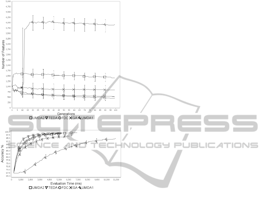
Figure 2: Dexter - Features vs Generations.
Figure 3: Dexter - Accuracy vs Classification Time.
case that in problems where effective feature sets are
small, fit solutions can only be found once the size
of the explored feature set has been substantially re-
duced. Due to the high level of noise in Dexter, de-
termining a useful probability distribution model for
a large set of candidate features of which only a few
are valid can be difficult.
In the initial population it is possible that some
small feature sets are generated by chance. Due to
the feature penalty, these are likely to have a better
fitness compared to other solutions in the population.
In a conventional EDA the large breeding pool may
obscure these solutions as they will have little effect
on the probability distribution. A GA may select such
solutions as one of its two parents and when it does so
it is likely to produce a smaller child solution. Whilst
GAs might by chance produce new solutions of the
same size as these small solutions, TEDA and FDC
do this explicitly and drive beyond the size of these
solutions to find even smaller feature sets.
UMDA2, which uses a smaller breeding pool and
mutation like a GA, is able to overcome the noise that
affects UMDA1 while taking advantage of the ability
of EDAs to exploit patterns within the population and
so proves very effective. This advantage that EDAs
demonstrate explains why TEDA outperforms FDC.
Classification Task: Arcene. The accuracies ob-
tained by selecting features for the Arcene classifica-
tion task are shown in figure 4. From these results, it
can be seen that FDC and TEDA both find better so-
lutions early on than the other approaches. UMDA2
starts to perform slightly better than these approaches
from around generation 25 onwards but for the first 10
generations it is completely unable to improve upon
the fittest individual in the initial population. UMDA1
is only able to start improving after about generation
70. The GA is also slower at finding good solutions
than TEDA and FDC, even though it is more effective
early on than UMDA.
By looking at the number of features used (fig-
ure 5) we can see that for both UMDAs the fittest
solution in the initial population has a median size
of 75 and that for a period of time both techniques
are unable to improve upon this. This is considerably
smaller than the maximum feature set size of 10,000
features. We can assume that the sizes of solutions in
the initial population is evenly distributed across the
range 1 to 10,000. Small individuals would be effec-
tively invisible to the probability model.
It would appear that the situation is the same for
both Arcene and Dexter. Initial high levels of noise
mean that until an algorithm starts to explore smaller
solutions all solutions are equally ineffective. A GA
might by chance select a small solution and breed a
new, similarly sized solution but TEDA accelerates
this process by making it explicit.
As with Dexter, figure 6 shows that these small
solutions can be classified more efficiently than larger
solutions and so, when plotted against time, we see
that TEDA and FDC have almost completed a 100
generation run before UMDA and the GA start to dis-
cover effective solutions.
Classification Task: Madelon. The results for the
Madelon classification task are shown in figures 7
to 9. In the Madelon problem both TEDA and
UMDA2 find good feature sets quicker than the other
techniques but UMDA1 eventually overtakes both
techniques. Both FDC and the GA are less effective.
A traditional EDA is more effective at this prob-
lem than the other problems possibly because the
need to dramatically reduce the size of feature set
does not apply in this case. The feature set size is
considerably smaller and there is less noise, so fea-
ture sets that use a large proportion of the available
features can be very effective. Figure 8 confirms this,
showing no steep declines or sudden drops in feature
ApplyingaHybridTargetedEstimationofDistributionAlgorithmtoFeatureSelectionProblems
141

Figure 4: Arcene - Accuracy vs Generations.
Figure 5: Arcene - Features vs Generations.
Figure 6: Arcene - Accuracy vs Classification Time.
set size as seen in the other problems. TEDA and
FDC show the greatest reduction in the size of feature
set and UMDA1 shows the least reduction as with the
Figure 7: Madelon - Accuracy vs Generations.
Figure 8: Madelon - Features vs Generations.
Figure 9: Madelon - Accuracy vs Classification Time.
other problems. Despite not reducing the feature set
size as fast or as far as for the other problems, plotted
against time (figure 9), TEDA is still able to find good
solutions earlier than the other techniques.
5 CONCLUSIONS
In this work we have shown the benefits of applying
TEDA to feature selection problems. We have tested
TEDA on three FSS problems from literature and in
all three cases it was able to find feature sets that were
both small and accurate in comparably quicker time
and less effort than standard EDAs and GAs. The
speed with which TEDA finds these small solutions
enables it to complete fitness function evaluations at
a faster rate than comparable algorithms. TEDA is
therefore a suitable algorithm for problems that have
a large number of features and where fitness function
evaluations are time consuming.
IJCCI2013-InternationalJointConferenceonComputationalIntelligence
142

Table 3: Seconds to Reach Accuracy Level.
Dexter
Acc. TEDA UMDA2 FDC GA UMDA1
70.0 0.29 0.3 0.31 0.34 1.65*
76.0 0.4 0.43 0.43 0.54* 2.73*
82.0 0.6 0.63 0.65 0.82* 4.02*
88.0 0.81 1.1* 0.92* 1.46* 6.16*
Arcene
70.0 2.06 3.44* 2.07 3.03* 26.42*
74.0 2.08 3.49* 2.11 3.11* 26.53*
78.0 2.12 3.49* 2.16 3.27* 26.68*
82.0 2.18 3.58* 2.21 3.38* -
86.0 2.28 3.69* 2.35 3.63* -
Madelon
70.0 23.54 24.79 24.02 23.52 30.67
74.0 39.98 35.74 50.0 52.19* 50.01*
78.0 52.43 67.28* 69.27 92.89* 96.97*
82.0 74.17 123.1* 106.58* 168.88* 175.93*
86.0 136.32 210.82* 200.73* 343.32* 270.93*
REFERENCES
Cantu-Paz, E. (2002). Feature subset selection by estima-
tion of distribution algorithms. In Proc. of Genetic and
Evolutionary Computation Conf. MIT Press.
Chang, C. C. and Lin, C. J. (2011). Libsvm: a library for
support vector machines. ACM Trans. on Intelligent
Systems and Technology (TIST), 2(3):27.
Dash, M., Liu, H., and Manoranjan (1997). Feature se-
lection for classification. Intelligent data analysis,
1:131–156.
Frank, A. and Asuncion, A. (2010). UCI machine learning
repository.
Godley, P., Cairns, D., Cowie, J., and McCall, J. (2008).
Fitness directed intervention crossover approaches ap-
plied to bio-scheduling problems. In Symp. on Com-
putational Intelligence in Bioinformatics and Compu-
tational Biology, pages 120–127. IEEE.
Guyon, I., Gunn, S., Ben-Hur, A., and Dror, G. (2004). Re-
sult analysis of the nips 2003 feature selection chal-
lenge. Advances in Neural Information Processing
Systems, 17:545–552.
Inza, I., Larranaga, P., Etxeberria, R., and Sierra, B.
(2000). Feature subset selection by bayesian networks
based on optimization. Artificial Intelligence, 123(1–
2):157–184.
Inza, I., Larranaga, P., and Sierra, B. (2001). Feature sub-
set selection by bayesian networks: a comparison with
genetic and sequential algorithms. Int. Journ. of Ap-
proximate Reasoning, 27(2):143–164.
Keller, J., Gray, M., and Givens, J. (1985). A fuzzy k-
nearest neighbor algorithm. IEEE Trans. on Systems,
Man and Cybernetics, 4:580–585.
Lai, C., Reinders, M., and Wessels, L. (2006). Random sub-
space method for multivariate feature selection. Pat-
tern Recognition Letters, 27(10):1067–1076.
Larranaga, P. and Lozano., J. A. (2002). Estimation of
distribution algorithms: A new tool for evolutionary
computation, volume 2. Springer.
Muhlenbein, H. and Paass, G. (1996). PPSN, volume IV,
chapter From recombination of genes to the estima-
tion of distributions: I. binary parameters., pages 178–
187. Springer, Berlin.
Neumann, G. and Cairns, D. (2012a). Targeted eda adapted
for a routing problem with variable length chromo-
somes. In IEEE Congress on Evolutionary Computa-
tion (CEC), pages 220–225.
Neumann, G. K. and Cairns, D. E. (2012b). Introducing in-
tervention targeting into estimation of distribution al-
gorithms. In Proc. of the 27th ACM Symp. on Applied
Computing, pages 334–341.
Pena, J., V. Robles, V., Larranaga, P., Herves, V., Rosales,
F., and Perez, M. (2004). Ga-eda: Hybrid evolutionary
algorithm using genetic and estimation of distribution
algorithms. Innovations in Applied Artificial Intelli-
gence, pages 361–371.
Pudil, P., J., Novovicova, and Kittler, J. (1994). Floating
search methods in feature selection. Pattern recogni-
tion letters, 15(11):1119–1125.
Saeys, Y., Degroeve, S., Aeyels, D., de Peer, Y. V., and
Rouz, P. (2003). Fast feature selection using a sim-
ple estimation of distribution algorithm: a case study
on splice site prediction. Bioinformatics, 19(suppl
2):179–188.
Siegel, S. and Jr., N. J. C. (1988). Nonparametric Statistics
for The Behavioral Sciences. McGraw-Hill, NY.
ApplyingaHybridTargetedEstimationofDistributionAlgorithmtoFeatureSelectionProblems
143
