Parameter Estimation and Equation Formulation in Business Dynamics

Marc Drobek

1,2

, Wasif Gilani

and Danielle Soban

SAP UK Ltd., Belfast, U.K.

Department of Mechanical and Aerospace Engineering, Queens University Belfast, U.K.

{marc.drobek, wasif.gilani}@sap.com, d.soban@qub.ac.uk

Keywords:

System Dynamics, Business Dynamics, Parameter Estimation, Equation Formulation, Non-linear Dynamic

Equations, Machine Learning, Big Data, Modelling, Classiﬁcation and Regression Trees.

Abstract:

System Dynamics enables modelling and simulation of highly non-linear feedback systems to predict future

system behaviour. Parameter estimation and equation formulation are techniques in System Dynamics, used

to retrieve the values of parameters or the equations for ﬂows and/or variables. These techniques are crucial

for the annotations and thereafter the simulation. This paper critically examines existing and well established

approaches in parameter estimation and equation formulation along with their limitations, identifying perfor-

mance gaps as well as providing directions for potential future research.

1 INTRODUCTION

As the world increases in complexity, so too do the

myriad systems that comprise it: from products such

as mobile phones and automobiles, to large and small

scale businesses, to our transportation system and

even to climate change. These complex systems can

be characterized as multi-dimensional, highly non-

linear, and containing dynamic feedback. The ﬁeld of

System Dynamics has long been used to model, un-

derstand, and predict the behaviour of these complex

systems. Business Dynamics, a specialized offshoot

of System Dynamics, has been particularly success-

ful in examining and analysing the complex business

models of todays commerce (Sterman, 2000). For

example, envision a business analyst whose goal is

to try and predict the behaviour of customers, par-

ticularly their trend in returning to business. Using

the Systems Dynamics approach, she starts by famil-

iarising herself with the business, including all im-

portant processes and strategic goals. She then col-

lects all inﬂuencing elements on the customer and

connects them together to create a meaningful Sys-

tems Dynamics model. After some reiterations and

further discussions with the process owners, prod-

uct managers, and customers, she ﬁnally has a suf-

ﬁciently accurate model to address the returning cus-

tomer scenario. Up to this point, she has leveraged

her skill and expertise in deﬁning and understanding

the problem, and has stayed well within her bound-

ary of knowledge and capability. The next critical

step, however, involves deﬁning the parameter values

and equations in her model, which drive the simula-

tions. Even though she has access to stored business

data, as well as some stock estimation techniques, she

still needs to manually determine the parameters and

equations in her model (Peterson 1976). This process

has traditionally been found to be time consuming,

cumbersome, resource intensive, and often necessi-

tates a level of mathematical and technical expertise

that may or may not be consistent with the analysts

basic knowledge set of the initial problem. In addi-

tion, by virtue of this process being a manual one, the

opportunity for error increases dramatically.

This process, called Parameter Estimation and

Equations Formulation (PEEF), is arguably the most

critical step in the entire modelling process, since it is

key to reliable and sufﬁcient system behaviour simu-

lations. But it is also one of the most challenging tasks

in the traditional System Dynamics process. This pa-

per begins with a survey of the state of the art ap-

proaches to parameter estimation and equation for-

mulation in a System Dynamics model. A detailed

overview of these concepts is provided, and advan-

tages and limitations are then summarized and dis-

cussed. The paper concludes by making a strong case

for the automation of the PEEF process, in order to ul-

timately improve the overall efﬁciency, accuracy, and

effectiveness of the System Dynamics approach.

166

Drobek M., Gilani W. and Soban D.

Parameter Estimation and Equation Formulation in Business Dynamics.

DOI: 10.5220/0004775101660176

In Proceedings of the Third International Symposium on Business Modeling and Software Design (BMSD 2013), pages 166-176

ISBN: 978-989-8565-56-3

2 BACKGROUND

This section contains a brief explanation of the Sys-

tem Dynamics concept. The authors introduce the

eight step modelling process by Burns, and discuss

PEEF.

2.1 Overview of System Dynamics

Concepts and Modelling Processes

The concept of System Dynamics has been widely ap-

plied to a large variety of ﬁelds, be it the simulation

and modelling of enterprises in ”Industrial Dynam-

ics” and city growth in ”Urban Dynamics” as shown

by (Forrester, 1961) and (Forrester, 1971), the world

population in ”Limits to Growth” (Meadows et al.,

1972), the System Dynamics National Model as sim-

ulation of social and economic change in countries

(Forrester et al., 1976) or the decline of the Mayan

empire in history (Hosler et al., 1977), among others.

These systems under study are highly non-linear dy-

namic systems which are continuously changing over

time. They consist of both static parameters, which

never change during each simulation run, and vari-

ables which may or may not change during simula-

tions. These parameters and variables are mostly in-

terdependent, meaning that there are circular depen-

dencies in the system under study. System Dynamics

modellers incorporate the circular dependencies by

modelling feedback loops to visualise cause and ef-

fect with causal loop diagrams (CLD) and/or state and

ﬂow diagrams (SFD). The ﬁgures 1 and 2 illustrate a

CLD and an SFD representing an economic problem

of returning customers, which also contains a feed-

back loop. A feedback loop in a system can either be

characterised as balancing or reinforcing. Balancing

loops drive the system behaviour sooner or later to-

wards a steady state, thus equilibrium, whereas rein-

forcing loops emphasise the growth itself, either pos-

itive or negative in each iteration of the loop. The

CLD and SFD are widely accepted in the System Dy-

namics community and support the modellers under-

standing of the system under study, as explained by

Lane (Lane, 2000). Whereas the CLDs main purpose

focusses on the identiﬁcation of basic elements (quan-

tities) and their connections (couplings) in the system

under study, the SFD is used to map the system to

a set of stocks (levels), rates, variables (auxiliaries),

constants (parameters), ﬂows and connections (infor-

mation couplings). The SFD, furthermore, visualises

the resources or materials ﬂowing through the system

under study. Such resources/materials are determined

by the system and might be, for instance, money, pol-

lution, population, water or customers as explained in

Figure 1: A causal loop diagram (CLD).

the introduction example. The previously mentioned

System Dynamics model types CLD and SFD have

been formally deﬁned by Burns (Burns, 1977), who

relied on the concept of set theory to provide for-

mal deﬁnitions of all elements. The steps involved in

modelling a speciﬁc system using the System Dynam-

ics approach have been discussed for decades (Burns,

1977; Ford, 1999; Binder et al., 2004). Burns gave

the following procedure:

1. Determine the concrete problem which shall be

modelled and the system boundaries.

2. Identify quantities in the system which reﬂect the

system (e.g. by considering smaller components

of the system) .

3. Blue-print the causal diagram by addressing de-

pendencies of previous deﬁned quantities using a

set of connections.

4. Migrate the causal diagram into a schematic

(ﬂow) diagram to highlight the resources or ma-

terial ﬂowing through the modelled system.

5. Formulate the model equations and estimate pa-

rameters with the help of the schematic diagram

and expert knowledge.

6. Transform equations into a machine program to

simulate the model.

7. Run the simulation and verify/validate the simula-

tion output with observed or expected real world

behaviour of the system.

8. Gain insights of simulation output, identify possi-

ble consequential policies and give client recom-

mendations.

In the early days of System Dynamics, Forrester

was for instance starting the modelling process with

an SFD and used the CLD close to the end of a

whole modelling process to summarise and visualise

the dominant loops in the current model. But later

Parameter Estimation and Equation Formulation in Business Dynamics

167

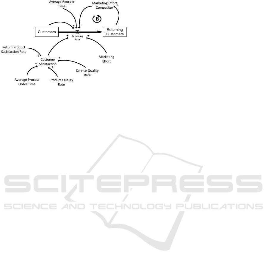
Figure 2: An economical state/ﬂow diagram (SFD).

on it was stated by other researchers, e.g. Haraldsson

(Haraldsson, 2000), that it might come handier to start

with the CLD to get a better understanding of the in-

volved quantities and their connections. Even though

the order of the previously deﬁned modelling process

might change from time to time, the general process

of modelling is still valid after more than 40 years.

2.2 PEEF (Parameter Estimation and

Equation Formulation)

The System Dynamics modeller has to rely upon a

huge knowledge base to identify the systems main

connections and the way in which the quantities are

inﬂuencing each other. Forrester stated that the qual-

ity of one model highly depends on the usage of

all known information about the system under study

(Forrester, 1991). This statement also holds for an-

notating a created SFD model with parameters and

equations. He divided the types of available knowl-

edge into three different classes, namely the mental

data base (experience and knowledge of humans), the

written data base (natural language text, written in-

structions) and the numerical data base (numbers in

a table). It was stated in the introduction section

that one of the critical phases in System Dynamics

is the computation of parameters and equations in the

model. There are existing approaches in place that

address this phase. However, these approaches either

lack automation, are very focussed towards speciﬁc

problems or are unable to fully exploit all available

data. Therefore, a clear potential exists for ground-

breaking research on ”Equation formulation and pa-

rameter estimation”, which corresponds to step 5 in

the traditional modelling process (see previous sec-

tion). The authors believe that PEEF is one of the ma-

jor requirements to systematically run the simulations

and predict model behaviour. Furthermore, the pro-

cess should be automatically supported and it should

be able to leverage all available data sources. The

available memory and computation power, which un-

til recently were considerable constraints to an auto-

mated process, are no longer an issue with the current

availability of cloud infrastructures and data centres.

Leveraging this new technology allows the modeller

to use all resources that might necessarily support her

in creating accurate simulation output.

3 STATE OF THE ART

This section discusses System Dynamics with respect

to PEEF, which is, after roughly 40 years, still mostly

manually done by the modeller. Relying on modeller

experience, assumptions and the knowledge of do-

main experts, if available, the initial parameters and

equations of resulting models are usually not provid-

ing satisfactory results after simulating the model. In

most cases, eventually a series of try (adjust parame-

ters/equations) and fail (rerun the simulation) replays

will deliver acceptable results in the end (see (For-

rester, 1991; Graham, 1981; Richardson, 1992)), but

this trial and error process is expensive and inefﬁcient.

Nonetheless a lot of excellent research has been done

in these ﬁelds (Senge, 1974; Peterson, 1976; Burns,

1977; Graham, 1980; Chen and Jeng, 2002; Medina-

borja and Pasupathy, 2007). To simplify further ex-

planation of these concepts, we will borrow the deﬁ-

nition of a very simple system from Peterson.

X(t) = A ∗ X(t − 1) +W (t) (1)

Z(t) = X (t) +V (t) (2)

Let X be the state of the system, A an unknown

parameter which has to be estimated, Z the actual

measured state of the system, W the equation error

(driving noise) and V the measurement error. Addi-

tionally

Z is deﬁned as the simulated state of the sys-

tem. In the now following subsections, we are going

to summarise the approaches of the former named re-

searchers.

3.1 Estimation through Simulation

The concept of imitating a real-world process over

time, so called simulation, is widely used in a variety

of technical ﬁelds, such as aeroplane design, build-

ing constructions, weather forecast etc. It is also one

of the common methods for parameter estimation in

System Dynamics. Senge and Peterson showed the

estimation of a parameter A by consecutively rerun-

ning the system simulation with new assumptions of

A until the simulation produces satisfying results. Pe-

terson called this method the Naive Simulation (NS).

Third International Symposium on Business Modeling and Software Design

168

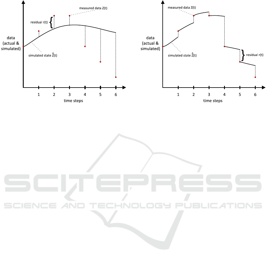
Figure 3: The naive simulation.

It is mostly accomplished by determining an initial

value for the parameter A (e.g. by guessing), run-

ning the simulation to get new results

Z, calculating

the difference between

Z and Z (so called residuals r)

and ﬁnally repeating this methodology until a value

for A has been found which causes the simulation

to produce acceptable results. To measure the suc-

cess of the parameter estimation, they were initially

using the Least squares method invented by Gauss

(Aldrich, 1998). This statistical concept is mostly

used in over-determined systems with more equations

than variables to estimate. The idea is to minimise

the sum of all squared residuals to get the best ﬁt for

the estimated parameter. Figure 3 shows an exam-

ple simulation and the residuals to be minimised with

the least squares approach. The NS approach works

very well in perfect systems not being inﬂuenced by

external circumstances (reﬂected in the equations as

driving noise W ). In fact Peterson has shown that

for systems containing driving noise W the NS ap-

proach might deliver completely wrong parameter es-

timations, because most of the available data is sim-

ply ignored and the system might completely drift

away from the simulation result (Peterson, 1975). In

such cases where driving noise is present, but mea-

surement errors are still absent, an advanced NS ap-

proach might deliver better results. Whenever a new

data point is available, Peterson referred to the Ordi-

nary Least Squares (OLS) method to reset the current

system state when simulating to counteract the drift

(Peterson, 1976). The method delivers satisfying re-

sults for modelled systems with driving noise W , but

it is easy to understand that measurement errors V of

each available data point will also end in unsatisfy-

ing parameter estimations due to the wrong state of

the system when resetting the system. One can ar-

gue that nowadays the quality of stored data in ware-

Figure 4: The ordinary square simulation.

houses and data bases is considerably more accurate

than back in the days, but at the time Peterson formu-

lated these ideas, stored data was rare and mostly not

checked automatically for quality or the observed data

was even retrieved manually. An excellent idea of

preventing the problem of high inﬂuence from mea-

surement errors to the estimation of parameter A is Pe-

tersons idea of the Full-Information Maximum Likeli-

hood (FIMLOF) algorithm. It is based on the Kalman

ﬁltering technique (Kalman, 1960). FIMLOF was de-

signed to determine the most likely state of the system

at each time t where data is available, by considering

all given measured, simulated and expected error data.

Whereas the measured and simulated data will be the

same input as by NS and OLS, the expected error data

is additionally computed by using the standard devia-

tion for the predicted state

Z and the variance for the

measured data Z. Given the two most likely cases

that either V is high and W is low (high measurement

errors, but low driving noise) or V is small and W is

high (the prediction is incorrect, but the observed data

has high quality) the algorithm will behave as follows:

In the ﬁrst case, FIMLOF will choose a value close to

the predicted output for the current time step, whereas

in the second case, the algorithm tends to choose a

value close to the measured data point. Either way,

FIMLOF has a very high chance to choose the most

likely value of the current system for the next simula-

tion step. This speciﬁc characteristic increases the ac-

curacy of the parameter estimation, because the more

accurate the predicted system state can be retrieved,

the fewer errors are passed through the parameter esti-

mation. Nevertheless, each of these approaches forces

the modeller to rerun the whole simulation several

times until ﬁnally computing a satisfying estimation

of parameter A. The simulation approach is therefore

no end-to-end process and works on hard assumptions

Parameter Estimation and Equation Formulation in Business Dynamics

169

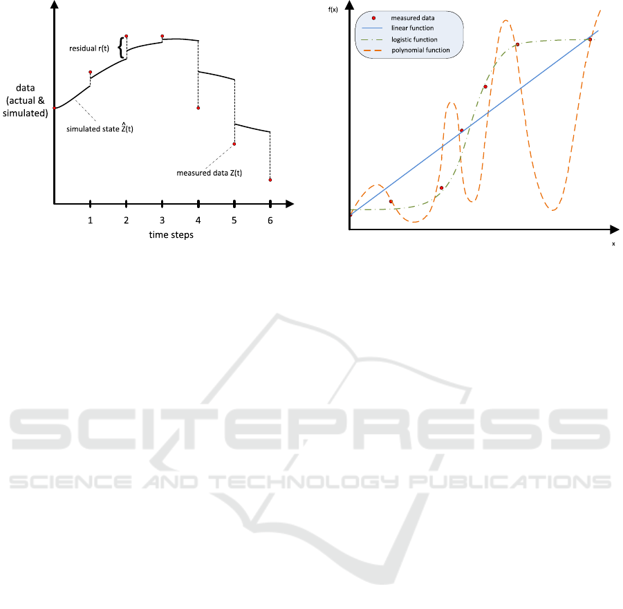
Figure 5: The FIMLOF simulation.

for the inital values of A, which is summarised in the

limitations L1 and L5.

3.2 Estimation by Data Type

Graham divided the model quantities into representa-

tions of data below the level of aggregation and data

at the level of aggregation (Graham, 1980). Data be-

low the level of aggregation (also called disaggregated

data) refers to observations and measurements made

in the real world which can be directly addressed and

therefore conforms to a speciﬁc observable character-

istic. Examples are the number of sold items in a mar-

ket at a speciﬁc time or the amount of vacation days

of one speciﬁc employee in a year. On the other hand,

data at the level of aggregation describes quantities

which are accumulated out of a number of different

basic values and are not atomic, e.g. the time for a

TCP/IP packet sent from one client machine to an-

other client machine. The main problem with data at

the level of aggregation is that it hides the main root

causes which are driving and inﬂuencing the aggre-

gated data. Graham shows different approaches of pa-

rameter estimation for data below the level of aggre-

gation and data at the level of aggregation (Graham,

1980).

The actual approach for estimating parameters

from disaggregated data depends on the available ob-

served data. If few data points are observed, the mod-

eller is able to determine a parameter by choosing a

value between the given observed limits. Dependent

on the size of the limit interval, the modellers guess

of parameter A might be more or less accurate. For

more available data points, Graham proposed to use

a table function with speciﬁc interpolations to deter-

mine the parameter A. The trick in this case is to iden-

tify the right interpolation to get slopes with smooth

Figure 6: Equation calculation with statistical analyses like

regression.

curves between the normal observed values and the

extreme observed values. And last, if the modeller

has access to numerical estimates or process obser-

vations which represent the modelled quantity, this

data might be used to calculate the actual value of

the modelled quantity. Graham uses the example of

the rabbit birth rate in an ecological model to explain

this methodology. Even though the modeller might

not have an observed value for the rabbit birth rate it-

self, she is at least in the position to acquire observed

behaviour about rabbit reproduction to calculate the

rabbit birth rate. In every case, parameter estima-

tion for disaggregated data never uses actual model

equations to retrieve parameters but instead relies on

statistical approaches like regression (linear or poly-

nomial). Figure 6 shows that by using statistical ap-

proaches an optimal ﬁt for a given data set might be

computed, but without background knowledge about

the analysed data set the resulting function might be

completely misleading for future data points. This

problem is covered with limitation L4 and fully ap-

plies to the concept of estimation via disaggregated

data.

Graham additionally explains the concepts of

Equation estimation and Model estimation to estimate

parameters from aggregated data. Both methods rely

on model equations and transposition (usage of alge-

bra) to estimate the parameters. Using equation esti-

mation, the modeller manipulates exactly one model

equation which consists of aggregated quantities like

stocks, ﬂows and variables to compute a value for one

parameter A. The methodology of model estimation

involves transposition of all model equations to cal-

culate parameters. In both cases, the modeller would

start to transpose the chosen model equation(s) up to

the point where A can be simply computed by insert-

Third International Symposium on Business Modeling and Software Design

170

ing the aggregated data values and resolving the equa-

tion(s). But working with aggregated data and model

equations usually involves assumptions made by the

modeller (see limitation L1), which in return gives

room for possible errors (Graham, 1980). However,

the quality of the parameter estimation for these meth-

ods is obviously highly dependent on the accuracy of

the underlying model equation(s) transposed and used

for calculation. Additional data of further involved

variables or rates, accessible by the modeller, is not

at all incorporated in the parameter calculation. This

approach is therefore only working on a possible frac-

tion of the available and accessible background data.

The two limitations L2 and L3 are described in the

limitation section.

3.3 Equations by Dimensions

Burns explained the approach of transforming a pre-

viously created causal diagram D (as in ﬁgure 1) into

a state/ﬂow model by using a square ternary matrix

(STM) and modiﬁed square ternary matrix (MSTM)

as intermediate steps (Burns, 1977). The STM con-

tains all quantities q

as rows and q

as columns of

a given causal diagram and deﬁnes either −1, 0 or 1

for a connection from q

to q

or no connection (usu-

ally empty cells), as shown in table 1 for the example

of the returning customers. The sign in front of a 1

indicates the inﬂuence of q

to q

, which is either neg-

ative or positive. After identifying a set of deﬁnitions

(D1 - D9) and a set of axioms (A1-A7) which reﬂect

the structure of a SFD according to Forrester, Burns

was able to create systematic algorithmic rules. These

rules, when applied to a STM, deliver an SFD. The

SFD might also be represented visually with a modi-

ﬁed STM (so called MSTM), as shown in table 3. The

MSTM differs from the STM in the representation of

the connections. Instead of having −1 and 1 as nega-

tive or positive connection, the MSTM contains either

−F, F or −I, I to indicate whether the represented

connection is an out- or inﬂow or a negative/positive

information coupling. Having the MSTM and the di-

mensions (dim) of each quantity enables the modeller

to retrieve equations for stocks, rates and variables

as follows. Stock equations are apparently trivial to

identify, because all stock equations are of the form:

calculate the difference between the inﬂow r

and the

outﬂow r

out

for the current time step ∆t and add this

value to the last value of stock x

, which translates to

the general equation:

(t + ∆t) = x

(t) + ∆t(r

− r

out

) (3)

The speciﬁc equations for each stock of a model

are therefore easily retrievable from the MSTM by

identifying the inﬂow and outﬂow of each stock. The

System Dynamics expert is furthermore able to de-

termine rate and variable equations by investigating

the MSTM and the dimensions (units) of these quan-

tities. Having a closer look to the MSTM columns

reveals the affecting quantities A

) for each vari-

able or rate quantity q

. As a matter of fact, q

has

to be at least calculated from its affected quantities,

otherwise the given causal diagram must have been

incorrect. Burns deﬁned this relation with equation 5

(see (Burns, 1977) pp. 705 for further information).

His mathematical function f is a mapping from all af-

fecting quantities q

∈ A

) to the quantity q

(see

equation 4).

f : Q

→ Q (4)

= f [{A

)}]

= f [{q

,. ..,q

}]

= q

⊗ ·· · ⊗ q

(5)

The goal of f is to establish dimension consis-

tency between all affecting quantities q

and the target

quantity q

. This is achieved by applying the math-

ematical operators (+, −, ∗, /), abbreviated by the

⊗ operator, to all affection quantities q

as shown in

equation 5. Because of the given mathematical oper-

ators, the equation deﬁned in f is always of a linear

form. This method apparently fails at the point when

some affecting quantities of q

are dimensionless or

the dimensions are not ﬁtting together. In this case,

Burns proposed to assume a table function for the af-

fecting quantities A

Apart from the limited linear form of the extracted

equations (see limitation L6), the expressions in each

equation are also not decorated with weighting fac-

tors and therefore might lead to inaccurate simulation

results. For example in the business world we can

easily build cases having one or more variables with

weighted dependencies: The price p and the quality q

of a product are both inﬂuencing the amount of sold

product units u

de f

, and can therefore be connected to

each other with the ⊗ operator as shown in equation

6. Since their dimensions are not ﬁtting, a table func-

tion T , which maps the result to product units, has to

be applied.

de f

= T (p ⊗ q) (6)

But dependent on the product, we can fairly as-

sume that either the price or the quality of the prod-

uct have more inﬂuence on the amount of sold units

and should be weighted with weights ω

and ω

. The

equation 7 shows the weighted connection of the price

and the quality,

wei

= T ((ω

∗ p) ⊗(ω

∗ q))

(7)

where ω

,ω

∈ [0,1.0] and ω

+ ω

= 1.0.

Parameter Estimation and Equation Formulation in Business Dynamics

171

Table 1: Square ternary matrix for the example of the re-

turning customers causal diagram.

dim 0 1 2 3 4 5 6 7 8 9 10

0 CO 1

1 CO 1

-1 1

-1

5 - 1

7 - 1

Table 2: Description of used dimensions.

abbreviation name description

CO customers the amount of

customers in the

system

TU time unit a unit of time rel-

ative to the over-

all system time

MU monetary

unit

standard currency

unit in the system

O orders all processed or-

ders

RP returned

products

all returned prod-

ucts in the sys-

tems

CC customer

complaints

all customer com-

plaints for orders

3.4 Equations with Surrogate Modelling

The sheer complexity of the System Dynamics do-

main including modelling, parameter estimation,

equation formulation, conﬁdence checking, etc., can

be addressed by borrowing ideas and techniques from

other well established domains.

Surrogate Modelling is one such potential inter-

disciplinary ﬁeld, which can be employed in the Sys-

tem Dynamics domain to address the complex equa-

tion formulation part. By blending the concepts from

the domains of Machine Learning and Statistics, Sur-

rogate Modelling offers a technique to create a surro-

gate function ˆg(x) for an unknown real function g(x)

by applying an analyses algorithm to a given train-

Table 3: Modiﬁed square ternary matrix for the example of

returning customers.

dim 0 1 2 3 4 5 6 7 8 9 10

0 CO I

1 CO I

-F F

-I

5 - I

7 - I

ing dataset. Dependent on the chosen analysis algo-

rithm different equations can be formulated, e.g. low-

order polynomials with the least-squares regression

algorithm, neural networks with a back-propagation

training algorithm or classiﬁcations with support vec-

tor machines. Since ˆg(x) is only a substitute of the

real function g(x), it does not necessarily produce the

same outputs for the same given inputs. A calcu-

lated surrogate function ˆg(x) might therefore be ei-

ther more accurate (computational intensive) or more

computational efﬁcient (less accurate) depending on

the given constraints (time, computation power, etc.).

Forrester et al. and Vapnik have provided an excellent

overview of Surrogate Modelling and available analy-

ses algorithms (Forrester et al., 2008; Vapnik, 1998).

However, research effort in this direction was initiated

by Chen & Jeng (Chen and Jeng, 2002) based on the

work of Dolado (Dolado, 1992). Chen and Jeng dis-

cussed the usage of artiﬁcial neural networks (ANN)

for System Dynamics as another representation of an

SFD in the ﬁrst place. ANNs were ﬁrst pioneered by

McCulloch & Pitts in the early 1940s and further im-

proved by Rosenblatts perceptron theory, Hopﬁelds

energy approach and Werbos back-propagation learn-

ing algorithm (McCulloch and Pitts, 1943; Rosen-

blatt, 1962; Hopﬁeld, 1982; Werbos, 1974). Chen and

Jeng used one partial recurrent neural network (PRN)

to represent a complete system dynamics model and

introduced a transformation from SFD to PRN. To en-

able such a transformation, there has to be a mapping

of System Dynamics elements (quantities and con-

nections) to neural network elements as follows. A

stock variable is transformed into an input, state and

output neuron. The input and output unit handle the

Third International Symposium on Business Modeling and Software Design

172

input and output function of a stock, whereas the state

unit serves as storage. Flows and their rates are repre-

sented by a hidden unit and the connection between a

hidden unit and an output unit, which is part of a stock

representation. Auxiliary variables are not mapped as

such, because Chen and Jeng argue that these vari-

ables might be expressed as subdivided parts of a rate

equation (”a rate in front of another rate” (Chen and

Jeng, 2002)). Furthermore, parameters (constants) are

either imitated with stocks without having a connec-

tion to hidden neurons to prevent changes in the sim-

ulation or parameters are treated as multipliers in rate

equations and therefore are not specially represented

with a neuronal network element. Finally informa-

tion couplings are illustrated with links between hid-

den and state neurons. Given these transformation

rules Chen and Jeng present a transformation algo-

rithm (FD2PRN) to convert a given SFD into a PRN.

They are furthermore applying standard algebra to the

activation functions of the PRN to proof the mathe-

matical compliance of the transformed PRN and the

typical stock, rate, initialisation and constant equa-

tions.

Up to this point the ANN is only used to illus-

trate any SFD and is therefore just another represen-

tation of a SFD like Burns MSTM. But as mentioned

earlier, ANNs have the ability to unveil hidden pat-

terns in a given dataset and therefore are capable of

providing predictions for the future development of

the dataset. The neural network mimics the equation

which produces the values of the given dataset. Hav-

ing this equation enables a modeller to predict future

values. In other words, if there is input data avail-

able for a given ANN, the ANN can be trained and

afterwards used to predict results. This statement also

holds for Chens & Jeng’s created PRN and they lever-

age this concept by training the raw untrained PRNs

of their System Dynamics test models with previously

simulated data. The trained PRNs might then be used

to predict the system behaviour, similar to simulation

runs of SFDs. The results for training of the PRN in

their paper are quite promising and given the learn-

ing ability of ANNs, they are highly adjustable to ex-

ternal changes in the system under study. These in-

sights motivate for deeper research in this ﬁeld and

we, the authors, believe that the concepts of Surro-

gate Modelling and Machine Learning in general are

very well suited to tackle the problem of automated

PEEF in System Dynamics. We are especially high-

lighting this, because these concepts are embodying

the least of our addressed limitations. Nevertheless,

there are open questions arising from Chen & Jengs

work. For instance, the prediction accuracy for known

worse neural network equations like alternating be-

haviour might not be appropriately represented by a

neural network.

3.5 Formulation via Decision Trees

For decades the System Dynamics community relied

on Forresters recommendations of the three different

models explained in the beginning of this paper on

how to retrieve knowledge for building System Dy-

namics models. Forrester values the mental model

far above the written and numerical model, because

there was simply not enough data to replace the hu-

man mind of the modeller and domain experts. This

guideline is still valid, but in the modern business

world where every digital step of each customer is

monitored and stored in huge databases, the written

and numerical models are becoming more and more

useful and relevant. Research communities in the area

of business intelligence and business process manage-

ment are exploiting this huge amount of available data

and proposing enhanced solutions in the area of busi-

ness decision support. For instance, Medina-borja &

Pasupathy are leveraging this data for semi-automated

model creation and equation formulation (Medina-

borja and Pasupathy, 2007). They are showing two

statistical approaches to identify predictors of model

variables from a given data set and afterwards one

algorithm to leverage these dependencies and reveal

their mathematical representations. Classiﬁcation and

Regression Trees (CART) and Chi-Square Automatic

Interaction Detection (CHAID) are both decision tree

methods which are used to divide the given data set

into groups and subgroups to assign them to nodes.

After the tree has been grown and possibly pruned,

most of the remaining nodes in the tree represent im-

portant independent variables. Common usages in the

literature for CART and CHAID are the identiﬁca-

tion of predictors for customer behaviour and market

segmentation, direct marketing to group customers

in classes or the ﬁeld of processing mining to clas-

sify process instances. On the other hand Structural

Equation Modelling (SEM) is a statistical approach

of validating or exploring a predeﬁned model with

a given data set, see for instance (Hayduk, 1985) or

(Pearl, 2000). One idea to use SEM is to ﬁrst cre-

ate a model which supposedly ﬁts the given data set

and afterwards applying the SEM algorithm to the de-

ﬁned model and given data set to ﬁgure whether the

model ﬁts the data and if so, how much. The model

consists of measured variables (indicators) and unob-

served/abstract variables (latent variables). The out-

come of SEM is the cause and effect sizes (structural

coefﬁcients) which might be used for equation for-

mulation. The idea proposed by Medina-borja & Pa-

Parameter Estimation and Equation Formulation in Business Dynamics

173

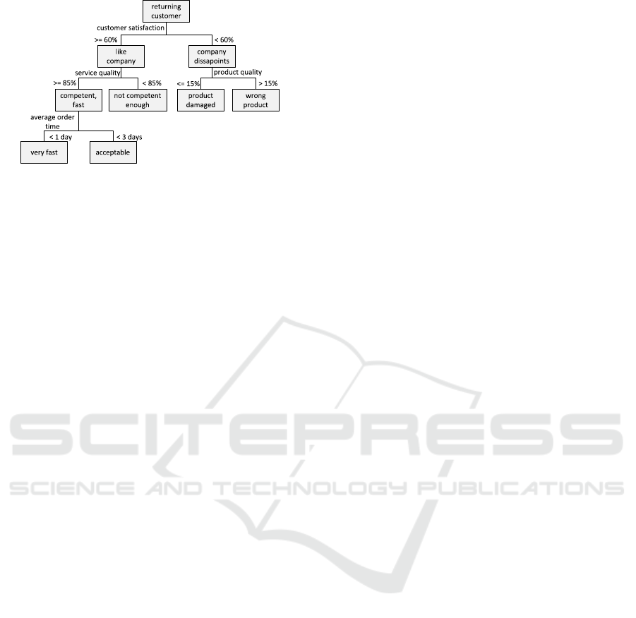
Figure 7: A regression tree for the problem of returning

customers.

supathy is to use CART or CHAID to uncover the de-

pendencies of a given data set and create a model us-

ing the generated decision tree. Afterwards SEM can

be used to determine the ﬁt of the model to the data

and to provide the structural equations of the model.

The resulting model and its equations can be used as

a SDM and eventually fed into simulation/analyses

tools. Unfortunately SEM is only capable of creat-

ing linear structural equations and is thus subject to

limitation L6. However this concept shows a semi-

automated procedure from a given data set to ﬁnal

simulation results.

4 GENERAL LIMITATIONS

All of the above stated approaches are extremely

helpful for a System Dynamics expert to either

retrieve parameter values or gain help in formulating

equations in a System Dynamics model. As each of

these concepts require speciﬁc prerequisites, there

are certain minor or major limitations associated

with these algorithms and additional questions arise

which need further research to be answered. We have

identiﬁed and collected a number of these limitations

(L1 - L6) which are either stated by the authors of the

algorithms themselves or are obvious when applying

the algorithms.

L1. Assumptions. We have observed that some of the

algorithms are working with hard assumptions, for in-

stance to guess initial values. Assumptions generally

lead to errors because there is always room to spec-

ulate. This limitation also implies a decrease in the

quality of the retrieved parameters/equations.

The algorithm works on assumptions.

L2. Predeﬁned Equations. The availability of System

Dynamics model equations is a strong prerequisite for

simulations. For instance, in the case of the estimat-

ing by data type approach, model equations have to

be manually provided to start transposing them and

ﬁnally resolving parameters. This possesses a sig-

niﬁcant limitation for the applicability of the algo-

rithm, because the equation formulation requires a

huge amount of effort and domain expertise. Given

the fact that the modeller is particularly interested in

the simulation result output, she is forced to addition-

ally perform the complex equation retrieval process

by hand.

Model equation information needed by the algorithm

restricts its usage and forces the modeller to deal

with additional intermediate steps.

L3. Limited Data Utilisation. Many of the algo-

rithms have a very restricted view on the available

data sets; they only consume a fraction of the avail-

able data. Good examples are observed in the equa-

tions by dimensions algorithm where only the dimen-

sions of all quantities are incorporated and in the esti-

mation through simulation algorithm where only the

historical measured data sets are captured. Histori-

cal measured data, for instance in the equations by

dimensions approach could be readily used to further

reﬁne the retrieved equations with weights. The lim-

ited data view drives towards inaccurate equation for-

mulations and thereby misleading simulation results.

Limited data utilisation leads to inaccurate equation

formulations.

L4. Interpolation. Many algorithms (especially sta-

tistical algorithms) are very much capable of provid-

ing optimal equations that ﬁt a given data set (see

polynomial regression algorithm ﬁgure 6). However,

these algorithms do not incorporate the actual seman-

tics hidden in the data while interpolating a given data

set. The resulting equations are therefore lacking the

accuracy to compute future data points outside the

given data set range.

The algorithm does not capture hidden patterns and

semantics.

L5. Automation. None of the algorithms support an

automated end-to-end process for PEEF. When us-

ing these algorithms, there are always intermediate

manual steps involved. For example, determining

the interpolation approach, aggregating data, provid-

ing basic equations for further reﬁnement, creating a

model from a given decision tree, training the algo-

rithm. Manual execution of an algorithm or inter-

vention while the algorithm is executed is not only

tedious and requires a lot of domain knowledge, but

also slows down the actual process and raises addi-

tional possibilities for failures.

Third International Symposium on Business Modeling and Software Design

174

Table 4: Overview of concepts for PEEF and their limitations.

Method Algorithm Type L1 L2 L3 L4 L5 L6

Simulation NS PE X X ◦ ◦ X n.a.

OLS PE X X ◦ ◦ X n.a.

FIMLOF PE ◦ X ◦ - X n.a.

Data type (disaggregated) Estimate between limits PE X - X X X n.a.

Estimate table functions PE X X ◦ X X n.a.

Calculate numerical data PE ◦ X - X ◦ n.a.

Data type (aggregated) Equation estimation PE X X X X X n.a.

Model estimation PE ◦ X ◦ X X n.a.

Dimension STM/MSTM EF - - X X X X

Surrogate Modelling FD2PRN EF - - - - ◦ -

Decision trees CART, CHAID, SEM EF ◦ - - ◦ ◦ X

The algorithm is not designed to operate in an

end-to-end fashion without manual intervention.

L6. Non-linearity. Linear equations can describe the

system properly, but as stated in L4 a wrongly se-

lected interpolation leads to inaccurate simulation re-

sults. Additionally, in the business world were we

have to deal with highly non-linear behaviour, algo-

rithms are needed, that are capable of computing non-

linear equations. A good example is that of the return-

ing customers (presented in ﬁgure 2). Since some of

its inﬂuencing factors, such as the average process or-

der time, can’t be written as independent linear com-

binations, the returning customers problem is a non-

linear system. The reason is that there are so many in-

ﬂuencing factors like marketing effort, the number of

one-time customers or even the average process order

time indirectly linked via customer satisfaction to the

returning rate. These variables and the ﬂow can more

precisely be captured with complex non-linear cubic,

logarithmic, exponential, etc. equations. We observed

that, not all analysed algorithms, which are intended

for equation formulation, are capable of producing the

non-linear equations that can optimally capture the

system behaviour.

The algorithm is not capable of extracting non-linear

equations.

All identiﬁed limitations are summarised in table 4.

For all analysed algorithms the following three sym-

bols are used to indicate how much the limitation ap-

plies to the current algorithm.

1. The hyphen symbol (-) implies that this limitation

does not apply at all.

2. A circle symbol (◦) suggests that this limitation is

partly valid.

3. The check mark symbol (X) shows that this limi-

tation completely holds.

The table contains a method column which de-

scribes the methodology used by the algorithm to

compute its results, an algorithm name, a type column

which either contains the abbreviation PE (parameter

estimation) or EF (equation formulation) to show the

main usage of the algorithm, and one column for each

deﬁned limitation, respectively.

5 CONCLUSIONS

In this paper the authors have analysed methodolo-

gies and techniques for PEEF in the domain of Sys-

tem Dynamics. These methodologies have facilitated

the work of System Dynamics modellers to run and

simulate the models and ﬁnally get output for future

system behaviour. Researchers like Burns, Graham

and Senge have developed concepts to estimate pa-

rameters and to formulate equations for System Dy-

namics models from the early 70s/80s. Neverthe-

less, each of the studied approaches is embodying

speciﬁc limitations which are posed by the very na-

ture of the concept itself or these approaches were

not originally meant to be used for PEEF in the ﬁrst

place. Especially for the equation formulation none

of the algorithms offers an end-to-end process from

model and data to annotated, ready to simulate model.

The authors believe that this concept of an end-to-

end automatic PEEF process is worthwhile to be re-

searched, because it would signiﬁcantly decrease the

manual workload of the modeller to retrieve param-

eters/equations. Chen & Jeng and Medina-borja &

Pasupathy have shown, that machine learning and

classiﬁcation approaches are very much suitable to

ﬁrst create the formal models and afterwards anno-

tate them with parameters and equations. Since nowa-

days more and more business data is generated and

stored, we see high potential especially in the surro-

gate modelling concepts to leverage this data for Busi-

ness Dynamics. Our future goal is to create a semi-

automated framework which is capable of transform-

ing business data into ready-to simulate SFDs. For

Parameter Estimation and Equation Formulation in Business Dynamics

175

this, we will have to incorporate an automated version

of PEEF within our planned framework. This will free

up the analyst from doing unnecessary tasks of man-

ual PEEF, allowing her to focus more on her actual

modelling tasks. We further plan to reuse and em-

bed the existing machine learning and classiﬁcation

approaches in our framework. We will invest further

research to help automate most of the crucial steps of

System Dynamics.

REFERENCES

Aldrich, J. (1998). Doing Least Squares: Perspectives

from Gauss and Yule. International Statistical Review,

66(1):61–81.

Binder, T., Vox, A., Belyazid, S., Haraldsson, H. V., and

Svensson, M. (2004). Developing System Dynamics

models from Causal Loop Diagrams. Technical re-

port, University of Luebeck, Germany; Lund Univer-

sity, Sweden.

Burns, J. R. (1977). Converting signed digraphs to For-

rester schematics and converting Forrester schematics

to Differential equations. IEEE Transactions on sys-

tems, man, and cybernetics, 10:695–707.

Chen, Y.-T. and Jeng, B. (2002). Yet another Representation

for System Dynamics Models , and Its Advantages. In

System Dynamics Society Conference.

Dolado, J. J. (1992). Qualitative Simulation and System

Dynamics. System Dynamics Review, 8(1):55–81.

Ford, A. (1999). Modeling the environment: An Intro-

duction to System Dynamics Models of Environmental

Systems. Island Press, Washington, D.C.

Forrester, A., Sobester, A., and Keane, A. (2008). Engi-

neering Design Via Surrogate Modelling: A Practical

Guide. Wiley-Blackwell.

Forrester, J. W. (1961). Industrial Dynamics. MIT Press;

currently available from Pegasus Communications;

Waltham, MA, Cambridge, MA.

Forrester, J. W. (1971). Urban Dynamics. Pegasus Com-

munications, Waltham, MA.

Forrester, J. W. (1991). System Dynamics and the Lessons

of 35 Years. pages 1–35.

Forrester, J. W., Mass, N. J., and Ryan, C. J. (1976).

The system dynamics national model: Understanding

socio-economic behavior and policy alternatives.

Graham, A. K. (1980). Parameter formulation and estima-

tion in System Dynamics Models. Elements of the Sys-

tem Dynamics Method, pages 143–161.

Graham, A. K. (1981). Lessons on modeling from the Sys-

tem Dynamics National Model. In 1981 System Dy-

namics Research Conference.

Haraldsson, H. V. (2000). Introduction to Systems and

Causal Loop Diagrams. Technical Report January,

Department of Chemical Engineering, Lund Univer-

sity, Lund.

Hayduk, L. A. (1985). The Conceptual and Measurement

Implications of Structural Equation Models. Cana-

dian Journal of Behavioural Science, 17.

Hopﬁeld, J. J. (1982). Neural Networks and Physical Sys-

tems with Emergent Collective Computational Abili-

ties. In In Proc. National Academy of Science, pages

2554–2558.

Hosler, D., Sabloff, J. A., and Runge, D. (1977). Simulation

model development: a case study of the Classic Maya

collapse. Academic Press: London.

Kalman, R. E. (1960). A new approach to linear ﬁltering

and prediction problems. Journal of Basic Engineer-

ing, 82:35–45.

Lane, D. C. (2000). Should System Dynamics be Described

as a ‘ Hard ’ or ‘ Deterministic ’ Systems Approach?

Systems Research and Behavioral Science, 22(June

1999):3–22.

McCulloch, W. S. and Pitts, W. (1943). A Logical Calculus

of Ideas Immanent in Nervous Activity. Bull. Mathe-

matical Biophysics, 5:115–133.

Meadows, D. H., Meadows, D. L., Randers, J., and Behrens,

W. (1972). The Limits to Growth. Universe Books,

New York, NY.

Medina-borja, A. and Pasupathy, K. S. (2007). Uncovering

Complex Relationships in System Dynamics Model-

ing: Exploring the Use of CART , CHAID and SEM.

In System Dynamics Society Conference, pages 1–24.

Pearl, J. (2000). Causality: Models, Reasoning and Infer-

ence. Cambridge University Press.

Peterson, D. W. (1975). Hypothesis, Estimation and Vali-

dation of Dynamic Social Models. PhD thesis, MIT,

Cambridge, Mass.

Peterson, D. W. (1976). Statistical Tools for System Dy-

namics. Elements of the System Dynamics Method,

pages 841–871.

Richardson, G. P. (1992). Problems for the Future of System

Dynamics. Technical report, Rockefeller College of

Public Affairs and Policy, University Albany.

Rosenblatt, R. (1962). Principles of Neurodynamics. Spar-

tan Books, New York.

Senge, P. M. (1974). An experimental evaluation of gener-

alized least squares estimation. In System Dynamics

Group Memo.

Sterman, J. D. (2000). Business Dynamics: Systems think-

ing and modeling for a complex world. McGraw-Hill,

New York, NY.

Vapnik, V. N. (1998). The Nature of Statistical Learning

Theory. Springer, 2nd edition.

Werbos, P. (1974). Beyond Regression: New Tools for Pre-

diction and Analysis in the Behavioral Sciences. PhD

thesis, Harvard University.

Third International Symposium on Business Modeling and Software Design

176