Shape Transformation of Multidimensional Density Functions

using Distribution Interpolation of the Radon Transforms

arton J

ozsef T

oth and Bal

azs Cs

ebfavi

Department of Control Engineering and Information Technology,

Budapest University of Technology and Economics,

Magyar tud

osok krt. 2, Budapest, Hungary

Keywords:

Shape-based Interpolation, Volume Morphing, Distribution Interpolation, Radon Transform.

Abstract:

In this paper, we extend 1D distribution interpolation to 2D and 3D by using the Radon transform. Our

algorithm is fundamentally different from previous shape transformation techniques, since it considers the

objects to be interpolated as density distributions rather than level sets of Implicit Functions (IF). First, we

perform distribution interpolation on the precalculated Radon transforms of two different density functions,

and then an intermediate density function is obtained by an inverse Radon transform. This approach guarantees

a smooth transition along all the directions the Radon transform is calculated for. Unlike the IF methods,

our technique is able to interpolate between features that do not even overlap and it does not require a one

dimension higher object representation. We will demonstrate that these advantageous properties can be well

exploited for 3D modeling and metamorphosis.

1 INTRODUCTION

Shape-based interpolation is mainly used for (1) mod-

eling or reconstruction of 3D objects from 2D cross

sections (Raya and Udupa, 1990; Herman et al., 1992;

Grevera and Udupa, 1996; Treece et al., 2000; Turk

and O’brien, 2002) and (2) morphing (Lerios et al.,

1995; Cohen-Or et al., 1998; Turk and O’Brien,

1999). The major application ﬁelds of these tech-

niques are Computer Aided Design (CAD), movie in-

dustry, and medical image processing and visualiza-

tion. In CAD systems, 3D geometrical models can be

built from contours deﬁned in cross-sectional slices

(Treece et al., 2000; Liu et al., 2008). Surfaces that

ﬁt onto the contours are obtained by using a contour-

interpolation method between the subsequent slices.

In the movie industry, shape transformation is used

for making special effects, such as morphing charac-

ters. In 3D medical imaging, it is usual that the reso-

lution of a volumetric data set is lower along the z axis

than along the x and y axes. Therefore, a shape-based

interpolation technique is applied to produce interme-

diate slices to obtain an isotropic volume represen-

tation (Raya and Udupa, 1990; Herman et al., 1992;

Grevera and Udupa, 1996; Treece et al., 2000). The

most popular way of automatic shape transformation

is based on an Implicit Function (IF) representation

of 2D or 3D shapes (Borgefors, 1986; Jones et al.,

2006). An intermediate shape is simply produced as a

level set of an IF that is calculated by interpolating be-

tween the IFs belonging to the initial and ﬁnal shapes

(Raya and Udupa, 1990; Herman et al., 1992). This

approach is easy to implement and robust in a sense

that topologically different shapes can be interpolated

without searching for pairs of corresponding points.

Nevertheless, in this paper, we show that the previous

IF methods are able to make a smooth transition be-

tween two features only if they are overlapping, oth-

erwise the features get disconnected. Furthermore,

shape-based interpolation of gray-scale images (in

other words, density functions) requires a one dimen-

sion higher representation than a shape-based inter-

polation of object boundaries (Grevera and Udupa,

1996). To remedy these problems, we propose a fun-

damentally different approach for shape-based inter-

polation. Our major goal is to guarantee a continu-

ous transition between the lower-dimensional projec-

tions of density functions to be interpolated. There-

fore, we precalculate the Radon transforms (Deans,

1983) of the density functions, which represent the

lower-dimensional projections from different angles,

and apply a distribution interpolation (Read, 1999)

between the corresponding projections. The result is

then transformed back by the classical Filtered Back-

Tóth M. and Csébfavi B..

Shape Transformation of Multidimensional Density Functions using Distribution Interpolation of the Radon Transforms.

DOI: 10.5220/0004640800050012

In Proceedings of the 9th International Conference on Computer Graphics Theory and Applications (GRAPP-2014), pages 5-12

ISBN: 978-989-758-002-4

 2014 SCITEPRESS (Science and Technology Publications, Lda.)

Projection (FBP) algorithm, which implements the in-

verse Radon transform. We will demonstrate that the

modeling potential of this algorithm is much higher

than that of the IF methods, as it is able to connect

features that do not overlap. Moreover, our method is

efﬁcient to use even for interpolating between 3D den-

sity functions, as the alternative representation pro-

duced by the Radon transform remains 3D, while

the classical shape-based interpolation of gray-scale

volumes would require 4D IFs to calculate (Grevera

and Udupa, 1996). Distribution interpolation and the

Radon transform are well-known tools that have been

used separately in different application ﬁelds, but to

the best of our knowledge, their combination and its

application for shape-based interpolation has not been

studied so far.

2 RELATED WORK

In computer graphics, shape-based interpolation is

usually applied for interpolating between the bound-

ary contours of 2D shapes or morphing between the

boundary surfaces of 3D objects. However, an au-

tomatic morphing between translucent objects (Kniss

et al., 2002), which are deﬁned by volumetric density

functions rather than explicit geometrical models is

still a challenging task. It depends on subjective pref-

erences whether a morphing algorithm should be fully

automatic or user-controlled. We think that the advan-

tages of these approaches are complementary and it

depends on the given application which one to prefer.

As we focus on automatic morphing, warping tech-

niques that require user intervention (Beier and Neely,

1992; Lerios et al., 1995; Cohen-Or et al., 1998; Fang

et al., 2000) are out of the scope of this paper. Auto-

matic morphing is favorable, for instance, if a shape-

based interpolation is required between all pairs of

consecutive slices in a huge volumetric data set, or a

morphing needs to be performed between 3D objects

that are completely different geometrically and corre-

sponding features can hardly be speciﬁed. The ma-

jor expectation from an automatic morphing method

is to provide intermediate objects that show features

of both objects which we interpolate between, and to

guarantee a smooth and gradual transition between

the features.

2.1 Shape-Based Interpolation of

Boundary Contours

Early shape-based interpolation techniques were pro-

posed for medical imaging applications, where the

goal was to reconstruct 3D shapes of different or-

gans from 2D slices of CT or MRI scans (Raya and

Udupa, 1990; Herman et al., 1992; Grevera and

Udupa, 1996). For example, this is a typical appli-

cation ﬁeld, where an automatic processing is clearly

an advantage, since a huge amount of voxel data is

required to be efﬁciently processed preferably with-

out any user interaction. As in a usual volumetric

data set the inter-slice distance is higher than the dis-

tance between the pixels of the slices, additional in-

termediate slices need to be interpolated to produce

an isotropic volume. The brute-force method is to

directly interpolate between the original slices, and

to apply the well-known Marching Cubes algorithm

(Lorensen and Cline, 1987) to extract a boundary sur-

face. However, this approach often results in severe

staircase artifacts. To reproduce smooth boundary

surfaces, shape-based interpolation techniques ﬁrst

detect boundary contours on the slices and then apply

a more sophisticated contour-interpolation method.

For contour interpolation, a variety of methods have

been published that build a triangular mesh which

connects the two consecutive contours (Bajaj et al.,

1996; Cheng and Dey, 1999; Treece et al., 2000; Liu

et al., 2008). Generally, this is a difﬁcult task, since

the problem of self-intersection and topologically dif-

ferent contours need to be carefully handled. Un-

like the direct contour-interpolation techniques, the IF

methods can easily avoid these problems. The basic

idea is to interpolate between the IFs that represent the

consecutive contours, and extract intermediate con-

tours from interpolated IFs. As a shape-based inter-

polation method is required to handle the distance

information somehow, it is a natural choice to use

a Signed Distance Map (SDM) as an IF (Borgefors,

1986; Jones et al., 2006). The pixels of a 2D SDM

represent the distance to the nearest contour point,

but inside the contour the sign is positive, while out-

side the contour it is negative. An intermediate con-

tour is obtained by extracting the zero-crossing level

set of the interpolated SDMs (Raya and Udupa, 1990;

Herman et al., 1992; Grevera and Udupa, 1996). The

SDM representation is efﬁcient to calculate using the

chamfering method (Akmal Butt and Maragos, 1998).

2.2 Shape-Based Interpolation of

Boundary Surfaces

Shape-based contour interpolation is straightforward

to extend to surface interpolation (Raya and Udupa,

1990). A boundary surface of an object can be rep-

resented by a 3D SDM, where the voxels store the

distance to the closest surface point. Similarly to

the 2D SDMs, the sign is positive inside the object

GRAPP2014-InternationalConferenceonComputerGraphicsTheoryandApplications

and negative outside the object. The interpolation

of the 3D SDMs and the extraction of the interme-

diate boundary surface are done analogously to the

2D case. Although this method can produce tran-

sitions between topologically different objects, the

transitions are often not smooth enough due to the

discontinuous curvature of the SDMs. In order to

achieve smoother transitions, variational interpolation

was proposed (Turk and O’Brien, 1999), which con-

structs IFs of minimal aggregate curvature. The IFs

are searched for as a linear combination of Radial Ba-

sis Functions (RBF) (Buhmann, 2009) and the coefﬁ-

cients are determined such that the curvature is min-

imized. This requires the solution of a large linear

equation system, which is time-consuming for com-

plex shapes. Furthermore, in case of such constrained

optimization problems, the coefﬁcient matrix is prone

to be ill-conditioned (Turk and O’brien, 2002); thus,

its inversion by the proposed LU decomposition could

easily become instable if the number of the unknown

variables drastically increase. This is probably the

reason why the variational interpolation (Turk and

O’Brien, 1999) has not been extended to gray-scale

images or volumes.

2.3 Extension to Gray-Scale Images and

Volumes

The shape-based interpolation of gray-scale images

(Grevera and Udupa, 1996) is computationally much

more expensive than the shape-based interpolation of

contours as it requires 3D IFs to interpolate rather

than only 2D IFs. Each image is considered to be

a height ﬁeld, which can alternatively be represented

by a 3D SDM. The intermediate images are obtained

as height ﬁelds extracted from the interpolated 3D

SDMs. Thus, both the chamfering and the extrac-

tion of the zero-crossing level set require the process-

ing of 3D volumes for each pair of consecutive im-

ages. A shape-based interpolation of gray-scale vol-

umes (Grevera and Udupa, 1996) is even more expen-

sive. Here, the height ﬁelds are deﬁned over the 3D

space; therefore, the corresponding SDMs are 4D data

sets. Consequently, 4D data processing is required to

obtain each single intermediate volume. The varia-

tional interpolation scheme (Turk and O’Brien, 1999)

has not been adapted to gray-scale images or volumes

yet, but using the same extension as for the SDMs,

it would also require a one dimension higher object

representation.

In contrast, our algorithm represents the gray-

scale images and volumes by their Radon transforms,

which are of the same dimensionality as the original

data. Additionally, we perform efﬁcient processing on

the Radon transforms; thus, all the computation can

be completed in a reasonable time. Moreover, as the

smoothness of the transition is guaranteed by the dis-

tribution interpolation on the projections the Radon

transform is evaluated for, a computationally expen-

sive constrained optimization (Cs

ebfalvi et al., 2002;

Neumann et al., 2002) is not necessary.

3 MULTIDIMENSIONAL

DISTRIBUTION

INTERPOLATION

In this section, we describe how to extend 1D distribu-

tion interpolation (Read, 1999) to higher dimensions

by using the Radon transform.

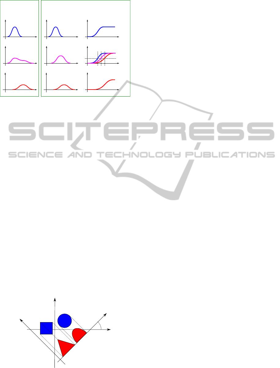
3.1 Distribution Interpolation in 1D

Let us assume that we have two 1D density functions

(x) and f

(x), and we want to interpolate between

them. For example, Figure 1 shows two Gaussian

density functions that are scaled and centered differ-

ently. In f

(x) the same amount of material is con-

centrated on the left side as in f

(x) on the right side.

Therefore, it is a natural expectation that this mass is

gradually moved from left to right in the intermedi-

ate interpolated density functions. Note that a simple

linear interpolation along the y axis clearly does not

fulﬁll this requirement. A distribution interpolation

(Read, 1999), however, does exactly what is expected

from a shape-based interpolation technique. Instead

of directly interpolating the density functions along

the y axis, this method actually interpolates the Cumu-

lative Distribution Functions (CDF) along the x axis.

The CDFs for f

(x) and f

(x) are deﬁned as follows:

(x) =

−∞

)dx

, (1)

(x) =

−∞

)dx

The ﬁrst step of the distribution interpolation is to ﬁnd

and x

such that F

) = F

) = y. The interpo-

lated CDF F

(x) takes the same value y at a linearly

interpolated position x = (1 − w)x

+ wx

. Positions

and x

are simply obtained by inverting the CDFs:

−1

(y) = x = (1 − w)x

+ wx

(2)

= (1 − w)F

−1

(y) + wF

−1

(y).

The interpolated CDF F

(x) is completely deﬁned by

its inverse function F

−1

(y), and the corresponding in-

terpolated density function is obtained by a simple

derivation:

(x) =

(x)

. (3)

ShapeTransformationofMultidimensionalDensityFunctionsusingDistributionInterpolationoftheRadonTransforms

density function

cumulative distribution function

x x

f (x)

F (x)

x x

f (x) F (x)

x x

f (x)

F (x)

x=(1-w)x + wx

distribution interpolation

w w

f (x)

linear interpolation

Figure 1: Distribution interpolation in 1D.

Figure 1 shows the interpolated density function for

w = 1/2. Distribution interpolation is usually applied

between probability density functions, so their inte-

grals are assumed to be equal to one. However, this

scheme can be easily adapted to mass distributions if

the distributions are normalized before the interpo-

lation and the interpolated distributions are rescaled

such that the a continuous transition of the total mass

is guaranteed.

3.2 The Radon Transform

Note that the 1D distribution interpolation cannot be

directly extended to higher dimensions. Since we pro-

pose an extension scheme that is based on the Radon

transform, here, we brieﬂy overview its evaluation

and inversion. The Radon transform (Deans, 1983)

of a 2D density function f (x,y) is deﬁned by a set of

1D projections p

(t):

(t) =

∞

−∞

∞

−∞

f (x,y)δ(x cos(θ)+y sin(θ)−t)dxdy,

(4)

where δ is the Dirac delta and θ is the projection an-

gle.

p (t)

f(x,y)

Figure 2: The Radon transform of a 2D density function is

deﬁned as a set of 1D projections p

(t).

The Radon transform is invertible, and its in-

verse can be evaluated by the classical Filtered Back-

Projection (FBP) algorithm (Kak and Slaney, 1988),

which consists of the following steps:

1. Fourier transform of the projections:

ˆp

(ν) =

∞

−∞

(t)e

−i2πtν

dt. (5)

2. Filtering in the frequency domain, where the fre-

quency response of the ﬁlter is |ν|:

ˆq

(ν) = ˆp

(ν) · |ν|. (6)

3. Inverse Fourier transform of ˆq

(ν):

(t) =

∞

−∞

ˆq

(ν)e

i2πtν

dν. (7)

4. Back-projection of the ﬁltered projections q

(t):

f (x,y) =

(x cos(θ) + y sin(θ))dθ. (8)

3.3 2D Distribution Interpolation

Now assume that we want to interpolate between two

2D density functions f

(x,y) and f

(x,y). In order to

guarantee that the projections of the interpolated den-

sity functions make a smooth transition between the

projections of f

(x,y) and f

(x,y), we apply distribu-

tion interpolation on the 1D projections rather than a

direct interpolation between the 2D density functions.

The Radon transforms of f

(x,y) and f

(x,y) are de-

noted by p

(t) and p

(t), respectively. A distribution

interpolation makes sense only if the projection func-

tions are normalized before. Therefore, we need to

calculate the integrals of f

(x,y) and f

(x,y):

∞

−∞

∞

−∞

(x,y)dxdy, (9)

∞

−∞

∞

−∞

(x,y)dxdy.

By using distribution interpolation between the nor-

malized projections p

(t)/s

and p

(t)/s

, we obtain

normalized intermediate distributions p

(t). To en-

sure a smooth transition of the total mass between

(x,y) and f

(x,y), the inverse Radon transform is

performed on rescaled projections p

(t)((1 − w)s

). The result of the inverse Radon transform is the

interpolated density function f

(x,y).

3.4 3D Distribution Interpolation

In order to interpolate between two 3D density func-

tions f

(x,y,z) and f

(x,y,z), 2D projections need to

be calculated:

GRAPP2014-InternationalConferenceonComputerGraphicsTheoryandApplications

(t,z) = (10)

∞

−∞

∞

−∞

(x,y,z)δ(x cos(θ) + ysin(θ) − t)dxdy,

(t,z) =

∞

−∞

∞

−∞

(x,y,z)δ(x cos(θ) + ysin(θ) − t)dxdy.

For a ﬁxed angle θ, p

(t,z) and p

(t,z) are, in fact,

2D density functions. Therefore, a 2D distribution in-

terpolation can be applied between them as described

in Section 3.3. Afterwards, an intermediate 3D den-

sity function f

(x,y,z) is reconstructed from the inter-

polated 2D projections p

(t,z) by using the standard

FBP algorithm, which is a de facto standard solution

for this classical tomography reconstruction problem.

In a practical implementation, a discrete approxima-

tion of the continuous integrals is applied. In order

to avoid a loss of information, it is required that the

total number of pixels in all discretized projections

is not smaller than the number of the voxels in the

discrete volumetric representations of the 3D density

functions.

4 APPLICATIONS

4.1 Shape-Based Interpolation of

Gray-Scale Images

Since our method is based on a Radon Transform

Interpolation, we refer to it as RTI. In contrast, the

method by Udupa and Grevera (Grevera and Udupa,

1996) is based on a Distance Transform Interpolation;

thus, we refer to it as DTI. We compare RTI to DTI

for the following reasons:

1. DTI is a de facto standard for an automatic shape-

based interpolation of gray-scale images.

2. DTI is a general solution and not designed for a

speciﬁc application ﬁeld.

3. Although for contour interpolation the varia-

tional framework of Turk and O’Brien (Turk

and O’Brien, 1999) provides smoother transitions

than the interpolation of SDMs, its extension to

gray-scale images is not trivial, and to the best of

our knowledge, has not been published so far.

Note that, using DTI, the chamfering results in just

an approximation of the Euclidean distance trans-

form. Although the approximation can be improved

by larger chamfering windows, it signiﬁcantly in-

creases the computational costs. Therefore, to make

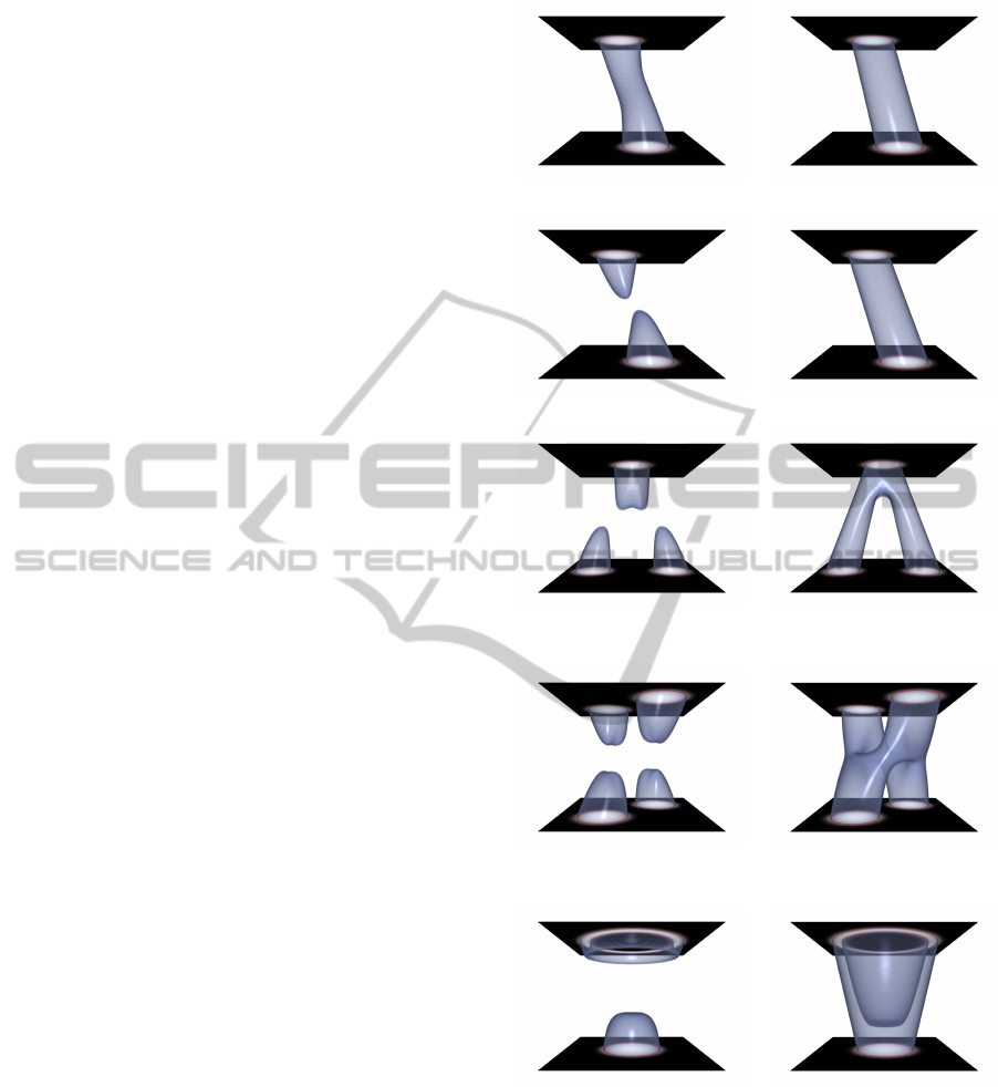
Interpolation between overlapping disc-shaped distributions.

Interpolation between non-overlapping disc-shaped distributions.

Transformation of one disc-shaped distribution

to two disc-shaped distributions.

Transformation of two disc-shaped distributions

to two other disc-shaped distributions.

Interpolation between disc-shaped and ring-shaped distributions.

Figure 3: Shape-based interpolation between different 2D

density distributions. Left: Interpolation of the distance

transforms. Right: Distribution interpolation of the Radon

transforms.

our comparison independent from the precision of the

distance transform, we evaluated the true Euclidean

distance maps for analytically deﬁned height ﬁelds,

which are interpreted as gray-scale images.

ShapeTransformationofMultidimensionalDensityFunctionsusingDistributionInterpolationoftheRadonTransforms

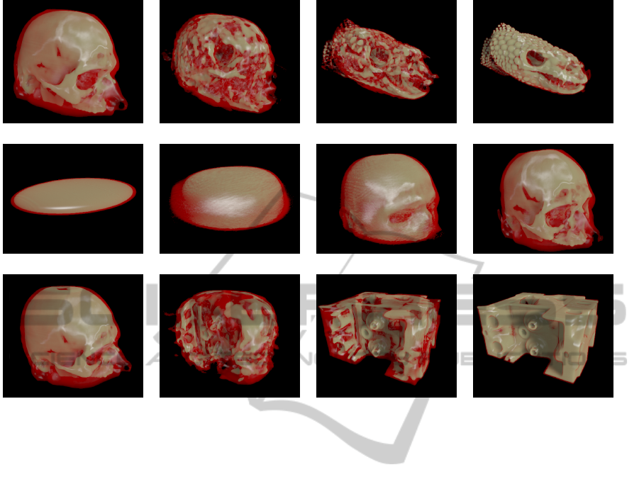
Figure 4: Automatic morphing between different gray-scale volumes using distribution interpolation on the Radon transforms.

Figure 3 shows several examples for shape-based

interpolations between different density distributions.

We generated 64 intermediate slices, and rendered the

resulting volume using direct volume rendering. The

ﬁrst example is the easiest one, where we interpolate

between two overlapping disc-shaped distributions.

Although DTI is able to make a connection, it also

produces an unexpected curvature. In contrast, RTI

results in a perfect tubular connection. In the second

example, only the distance between the disc-shaped

distributions is increased such that they do not over-

lap anymore. Note that, in this case, DTI fails to make

a connection, while RTI still provides a perfect transi-

tion. The third and fourth examples well demonstrate

that, unlike DTI, RTI can appropriately handle bifur-

cations. In the last example, again two density distri-

butions are interpolated, which do not overlap. DTI

cannot make a connection for this case either, while

RTI is able to connect the ring-shaped and disc-shape

density distributions forming a glass shape. These ex-

amples clearly show that RTI can be a reasonable al-

ternative of DTI, for instance, in a modeling applica-

tion.

4.2 Metamorphosis of Gray-Scale

Volumes

In order to test our method also on gray-scale vol-

umes, we implemented the entire algorithm on the

GPU using CUDA. Note that, all the processing steps,

such as the Radon transform, its inversion by FBP,

and the distribution interpolation of the 1D projec-

tions are easy to map onto the parallel architecture

of the GPU. For the frequency-domain ramp ﬁltering,

we used the CUDA FFT library. Figure 4 shows a

couple of examples for 3D morphing. For each pair

of volumes we generated 20 intermediate volumes of

resolution 256

, which took less than an hour on an

nVidia Tesla M2070 graphics card. In contrast, we

found it unfeasible to efﬁciently implement DTI for

gray-scale volumes on the GPU. Although there ex-

ist fast GPU implementations for calculating the dis-

tance transform in 2D or 3D (Schneider et al., 2009),

applying DTI, the shape-based interpolation of gray-

scale volumes would require 4D distance maps to cal-

culate. For example, using ﬂoating-point arithmetics,

for a volume of resolution 256

, the corresponding

4D distance map would take 256

× 4 = 16 Gbytes of

memory, which exceeds the capacity of recent graph-

ics cards. Furthermore, the calculation of such a huge

GRAPP2014-InternationalConferenceonComputerGraphicsTheoryandApplications

4D distance map would involve a signiﬁcant com-

putational cost. Variational interpolation (Turk and

O’Brien, 1999) is also very difﬁcult to extend to gray-

scale volumes. Using the extension scheme of Udupa

and Grevera (Grevera and Udupa, 1996), the gray-

scale volumes could be treated as height ﬁelds deﬁned

over the 3D space. Since these height ﬁelds can be

represented by 4D IFs, the shape transformation be-

tween them would require a 4D RBF interpolation. To

avoid the loss of ﬁne details, at least to each voxel a

4D RBF needs to be assigned. Thus, for a pair of vol-

umes with resolution 256

, the number of unknown

variables is 256

× 2. Consequently, the coefﬁcient

matrix of the corresponding linear equation system

contains 256

× 4 elements, which makes the inver-

sion practically impossible. Overall, we think that

compared to the computational and storage costs of

the previous methods, our soution is simple and efﬁ-

cient.

5 CONCLUSION

In this paper, we have introduced a novel algorithm

for shape-based interpolation of gray-scale images

and volumes. As far as we know, our technique is

the ﬁrst to combine distribution interpolation and the

Radon transform. The major advantage of this com-

bination is that the Radon transform does not require

a one dimension higher representation than the orig-

inal images and volumes. This is not the case for

the previous IF methods, where the gray-scale images

and volumes can alternatively be represented by 3D

and 4D IFs, respectively. Moreover, we demonstrated

that the distribution interpolation of the Radon trans-

forms can make a smooth connection between non-

overlapping features that the IF methods are typically

not able to connect. Due to this advantageous proper-

ties, we think that our method represents a signiﬁcant

contribution to the ﬁeld of shape-based interpolation.

ACKNOWLEDGEMENTS

This work was supported by projects T

AMOP-

4.2.2.B-10/1–2010-0009 and OTKA K-101527. The

Heloderma data set is from the Digital Morphology

(http://www.digimorph.org) data archive. Special

thanks to Dr. Jessica A. Maisano for making this data

set available to us.

REFERENCES

Akmal Butt, M. and Maragos, P. (1998). Optimum design

of chamfer distance transforms. IEEE Transactions on

Image Processing, 7(10):1477–1484.

Bajaj, C. L., Coyle, E. J., and nan Lin, K. (1996). Arbi-

trary topology shape reconstruction from planar cross

sections. In Graphical Models and Image Processing,

pages 524–543.

Beier, T. and Neely, S. (1992). Feature-based image

metamorphosis. SIGGRAPH Computer Graphics,

26(2):35–42.

Borgefors, G. (1986). Distance transformations in digital

images. Computer Vision, Graphics, and Image Pro-

cessing, 34(3):344–371.

Buhmann, M. (2009). Radial Basis Functions: Theory and

Implementations. Cambridge Monographs on Applied

and Computational Mathematics. Cambridge Univer-

sity Press.

Cheng, S.-W. and Dey, T. K. (1999). Improved construc-

tions of delaunay based contour surfaces. In Proc.

ACM Sympos. Solid Modeling and Applications 99,

pages 322–323.

Cohen-Or, D., Solomovic, A., and Levin, D. (1998). Three-

dimensional distance ﬁeld metamorphosis. ACM

Transactions on Graphics, 17(2):116–141.

ebfalvi, B., Neumann, L., Kanitsar, A., and Gr

oller, E.

(2002). Smooth shape-based interpolation using the

conjugate gradient method. In Proceedings of Vision,

Modeling, and Visualization, pages 123–130.

Deans, S. R. (1983). The Radon Transform and Some of Its

Applications. Krieger Publishing.

Fang, S., Srinivasan, R., Raghavan, R., and Richtsmeier,

J. T. (2000). Volume morphing and rendering - an

integrated approach. Computer Aided Geometric De-

sign, 17(1):59–81.

Grevera, G. J. and Udupa, J. K. (1996). Shape-based inter-

polation of multidimensional grey-level images. IEEE

Transactions on Medical Imaging, 15(6):881–92.

Herman, G. T., Zheng, J., and Bucholtz, C. A. (1992).

Shape-based interpolation. IEEE Computer Graphics

and Applications, 12(3):69–79.

Jones, M. W., Brentzen, J. A., and Sramek, M. (2006). 3D

distance ﬁelds: A survey of techniques and applica-

tions. IEEE Transactions on Visualization and Com-

puter Graphics, 12:581–599.

Kak, A. C. and Slaney, M. (1988). Principles of Computer-

ized Tomographic Imaging. IEEE Press.

Kniss, J., Premoze, S., Hansen, C., and Ebert, D. (2002).

Interactive Translucent Volume Rendering and Proce-

dural Modeling. In Proceedings of IEEE Visualization

Conference (VIS) 2002, pages 109–116.

Lerios, A., Garﬁnkle, C. D., and Levoy, M. (1995). Feature-

based volume metamorphosis. In Proceedings of the

22nd annual conference on Computer graphics and

interactive techniques, SIGGRAPH ’95, pages 449–

456.

Liu, L., Bajaj, C., Deasy, J., Low, D. A., and Ju, T. (2008).

Surface reconstruction from non-parallel curve net-

works. Computer Graphics Forum, 27(2):155–163.

ShapeTransformationofMultidimensionalDensityFunctionsusingDistributionInterpolationoftheRadonTransforms

Lorensen, W. E. and Cline, H. E. (1987). Marching cubes:

A high resolution 3D surface construction algorithm.

Computer Graphics, 21(4):163–169.

Neumann, L., Cs

ebfalvi, B., Viola, I., Mlejnek, M., and

oller, E. (2002). Feature-Preserving Volume Fil-

tering . In VisSym 2002 : Joint Eurographics - IEEE

TCVG Symposium on Visualization, pages 105–114.

Raya, S. and Udupa, J. (1990). Shape-based interpolation

of multidimensional objects. IEEE Transactions on

Medical Imaging, 9(1):32–42.

Read, A. L. (1999). Linear interpolation of histograms. Nu-

clear Instruments and Methods, A425:357–360.

Schneider, J., Kraus, M., and Westermann, R. (2009). GPU-

based real-time discrete euclidean distance transforms

with precise error bounds. In International Confer-

ence on Computer Vision Theory and Applications

(VISAPP), pages 435–442.

Treece, G. M., Prager, R. W., Gee, A. H., and Berman,

L. H. (2000). Surface interpolation from sparse cross-

sections using region correspondence. IEEE Transac-

tions on Medical Imaging, 19(11):1106–1114.

Turk, G. and O’Brien, J. F. (1999). Shape transformation

using variational implicit functions. In Proceedings of

ACM SIGGRAPH 1999, pages 335–342.

Turk, G. and O’brien, J. F. (2002). Modelling with im-

plicit surfaces that interpolate. ACM Transanctions

on Graphics, 21(4):855–873.

GRAPP2014-InternationalConferenceonComputerGraphicsTheoryandApplications