
A Pattern Recognition System for Detecting Use of Mobile Phones While
Driving
Rafael A. Berri
1
, Alexandre G. Silva
1
, Rafael S. Parpinelli
1
, Elaine Girardi
1
and Rangel Arthur
2
1
College of Techological Science, Santa Catarina State University (UDESC), Joinville, Brazil
2
Faculty of Technology, University of Campinas (Unicamp), Limeira, Brazil
Keywords:
Driver Distraction, Cell Phones, Machine Learning, Support Vector Machines, Skin Segmentation, Computer
Vision, Genetic Algorithm.
Abstract:
It is estimated that 80% of crashes and 65% of near collisions involved drivers inattentive to traffic for three
seconds before the event. This paper develops an algorithm for extracting characteristics allowing the cell
phones identification used during driving a vehicle. Experiments were performed on sets of images with 100
positive images (with phone) and the other 100 negative images (no phone), containing frontal images of the
driver. Support Vector Machine (SVM) with Polynomial kernel is the most advantageous classification system
to the features provided by the algorithm, obtaining a success rate of 91.57% for the vision system. Tests done
on videos show that it is possible to use the image datasets for training classifiers in real situations. Periods of
3 seconds were correctly classified at 87.43% of cases.
1 INTRODUCTION
The distraction whiles driving (Regan et al., 2008;
Peissner et al., 2011), ie, an action that diverts the
driver’s attention from the road for a few seconds, re-
presents about half of all cases of traffic accidents.
Dialing a telephone number, for example, consumes
about 5 seconds, resulting in 140 meters traveled by
an automobile at 100 km/h (Balbinot et al., 2011). In
a study done in Washington by Virginia Tech Trans-
portation Institute revealed, after 43, 000 hours of test-
ing, that almost 80% of crashes and 65% of near col-
lisions involved drivers who were not paying enough
attention to traffic for three seconds before the event.
About 85% of American drivers use cell phone
while driving (Goodman et al., 1997). At any day-
light hour 5% of cars on U. S. roadways are driven by
people on phone calls (NHTSA, 2011). Driver dis-
traction has the three main causes: visual (eyes off
the road), manual (hands off the wheel), and cogni-
tive (mind off the task) (Strayer et al., 2011). Talk-
ing on a hand-held or handsfree cell phone increases
substantially the cognitive distraction (Strayer et al.,
2013).
This work proposes a pattern recognition system
to detect hand-held cell phone use during the act of
driving to try to reduce these numbers. The main goal
is to present an algorithm for the characteristics ex-
traction which identifies the cell phone use, producing
a warning that can regain the driver’s attention exclu-
sively to the vehicle and the road. The aim is also
to test classifiers and choose the technique that maxi-
mizes the accuracy of the system. In Section 2 related
works are described. Support tools for classification
are presented in Section 3. In Section 4 the algorithm
for feature extraction is developed. In Section 5 ex-
periments performed on an image database are shown.
And finally conclusions are set out in Section 6.
2 RELATED WORKS
The work produced by (Veeraraghavan et al., 2007)
is the closest to this paper. The authors’ goal is to
make detection and classification of activities of a
car’s driver using an algorithm that detects relative
movement and the segmentation of the skin of the
driver. Therefore, its operation depends on obtaining
a set of frames, and the need to put a camera side-
ways (in relation to the driver) in the car, impeding
the presence of passengers beside the driver.
The approach of (Yang et al., 2011) use custom
beeps of high frequency sent through the car sound
equipment, network Bluetooth, and a software run-
ning on the phone for capturing and processing sound
411
A. Berri R., G. Silva A., S. Parpinelli R., Girardi E. and Arthur R..
A Pattern Recognition System for Detecting Use of Mobile Phones While Driving.
DOI: 10.5220/0004684504110418
In Proceedings of the 9th International Conference on Computer Vision Theory and Applications (VISAPP-2014), pages 411-418
ISBN: 978-989-758-004-8
Copyright
c
2014 SCITEPRESS (Science and Technology Publications, Lda.)

signals. The purpose of the beeps are to estimate the
position in which the cell phone is, and to differen-
tiate whether the driver or another passenger in the
car is using it. The proposal obtained accuracy clas-
sification of more than 90%. However, the system
depends on the operating system and mobile phone
brand, and the software has to be continually enabled
by the driver. On the other hand, the approach works
even if there is use of headphones (hands-free).
The study of (Enriquez et al., 2009) segments the
skin, analyzing two color spaces, YCrCb and LUX,
and using specifically the coordinates Cr and U. The
advantage is the ability to use a simple camera (web-
cam) for image acquisition.
Another proposal by (Watkins et al., 2011) is au-
tonomously to identify distracted driver behaviors as-
sociated with text messaging on devices. The ap-
proach uses a cell phone programmed to record any
typing done. An analysis can be performed to verify
distractions through these records.
3 PRELIMINARY DEFINITIONS
In this section, support tool for classifying classes are
presented.
3.1 Support Vector Machines (SVM)
The SVM (Support Vector Machine) was intro-
duced by Vapnik in 1995 and is a tool for bi-
nary classification (Vapnik, 1995). Given data set
{(~x
1
,y
1
),··· , (~x
n
,y
n
)} with input data ~x
i
∈ R
d
(where
d is the dimensional space) and output y labeled as
y ∈ {−1, +1}. The central idea of the technique is to
generate an optimal hyperplane chosen to maximize
the separation between the two classes, based on sup-
port vector (Wang, 2005). The training phase consists
in the choice of support vectors using the training data
before labeled.
From SVM is possible to use some kernel func-
tions for the treating of nonlinear data. The kernel
function transforms the original data into a space of
features of high dimensionality, where the nonlinear
relationships can be present as linear (Stanimirova
et al., 2010). Among the existing kernels, there are
Linear (Equation 1), Polynomial (Equation 2), Radial
basis (Equation 3), and Sigmoid (Equation 4). The
choice of a suitable function and correct parameters
are an important step for achieving the high accuracy
of the classification system.
K(~x
i
,~x
j
) =~x
i
·~x
j
(1)
K(~x
i
,~x
j
) = (γ(~x
i
·~x
j
)+coe f 0)
degree
,where γ > 0 (2)
K(~x
i
,~x
j
) = e
−γk(~x
i
+~x
j
)k
2
,where γ > 0 (3)
K(~x
i
,~x
j
) = tanh(γ(~x
i
·~x
j
) + coe f 0) (4)
We can start the training after the choice of the
kernel function. We need to maximize the values
for
~
α in Equation 5. This is a quadratic program-
ming problem (Hearst et al., 1998) and it is subject
to the constraints (for any i = 1, ..., n where n is the
amount of training data): 0 ≤ α
i
≤ C e
∑
n
i=1
α
i
y
i
= 0.
The penalty parameter C has the ratio of the algo-
rithm complexity and the number of wrongly classi-
fied training samples.
W (
~
α) =
n
∑
i=1
α
i
−
1
2
n
∑
i, j=1
α
i
α
j
y
i
y
j
K(~x
i
,~x
j
) (5)
The threshold b is found with Equation 6. The
calculation is done for all the support vectors ~x
j
(0 ≤
α
j
≤ C). The b value is equal to the average of all
calculation.
b = y
j
−
l
∑
i=1
y
i
α
i
K(~x
i
,~x
j
) (6)
A feature vector ~x can be classified (prediction)
with Equation 7, where λ
i
= y
i
α
i
and mathematical
function sign extracts the sign of a real number (re-
turns: −1 for negative, 0 for zero value and +1 for
positive values).
f (~x) = sign(
∑
i
λ
i
K(~x,~x
i
) + b) (7)
This SVM
1
uses imperfect separation, and the nu
is used as a replacement for C. The parameter nu uses
values between 0 and 1. If this value is higher, the
decision boundary is smoother.
4 EXTRACTION OF FEATURES
Driving act makes drivers instinctively and continu-
ally look around. But with the use of the cell phone,
the tendency is to fix the gaze on a point in front, ef-
fecting the drivability and the attention in the traffic
by limiting the field of vision (Drews et al., 2008).
Starting from this principle, this work choses an algo-
rithm that can detect the use of cell phones by drivers
just by using the frontal camera attached on the dash-
board of a car. The following subsections explain the
details.
1
The library LibSVM is used (available in
http://www.csie.ntu.edu.tw/∼cjlin/libsvm).
VISAPP2014-InternationalConferenceonComputerVisionTheoryandApplications
412

4.1 Algorithm
In general, the algorithm is divided into the following
parts:
Acquisition: Driver image capture system.
Preprocessing: Location of the driver, cropping the
interest region (Section 4.1.1).
Segmentation: Isolate the driver skin pixels (Sec-
tion 4.1.2).
Extraction of Features: Extraction of skin percen-
tage in regions where usually the driver’s
hand/arm would be when using the cell phone,
and calculation of HU’s Moments (Hu, 1962)
(Section 4.1.3).
In the following subsections, the steps of the algo-
rithm (after the image acquisition) are explained.
4.1.1 Preprocessing
After image acquisition, the preprocessing step is
tasked to find the region of interest, ie, the face of
the driver. In this way, three detectors
2
are applied
based on Haar-like-features for feature extraction and
Adaboost as classifier (Viola and Jones, 2001). The
algorithm adopts the largest area found by these de-
tectors as being the drivers face.
The region found is increased by 40% in width,
20% to the left and 20% to the right of the face be-
cause often this is much reduced (allows only the
face to be visible), becoming impossible to detect the
hand/arm. In Figures 1(a) and 1(c), preprocessing re-
sults are exemplified.
4.1.2 Segmentation
The segmentation is based on locating pixels of the
skin of the driver present in the preprocessed ima-
ge. It is necessary, as a first step, converting the
image into two different color spaces: Hue Satu-
ration Value (HSV) (Smith and Chang, 1996) and
Luminance–chrominance YCrCb (Dadgostar and Sar-
rafzadeh, 2006).
After the initial conversion, a reduction of the
complexity of the three components from YCbCr and
HSV is applied. Each component has 256 possible
levels (8 bits) resulting in more than 16 million pos-
sibilities (256
3
) by color space. Segmentation is sim-
plified by reducing the total number of possibilities
in each component. The level of each component is
2
Haar-like-features from OpenCV (http://opencv.org)
with three training files: haarcascade frontalface alt2.xml,
haarcascade profileface.xml and haarcas-
cade frontalface default.xml
divided by 32. Thus, each pixel has 512 possibilities
((
256
32
)
3
) of representation.
A sample of skin is then isolated with size of 10%
in the height and 40% in width of the image, being
centralized in the width and with the top in center of
the height, according to the rectangles in Figures 1(a)
and 1(c). A histogram with the 3 dimensions of HSV
and YCrCb skin sample from this region is created
by counting the pixels that have the same levels in all
3 components. Further, a threshold is performed in
the image with the levels that represent at least 5% of
the pixels contained in the sample region. Though the
skin pixels for HSV and YCrCb are obtained separa-
tely, the results are the pixels that are in both segmen-
tation of HSV and YCrCb. In Figures 1(b) and 1(d),
segmentation results are exemplified.
4.1.3 Features
Two features are part of the driver’s classification with
or without cell phone: Percentage of the Hand (PH)
and Moment of Inertia (MI).
PH is obtained by counting the skin pixels in two
regions of the image, as shown in red rectangles of
Figures 1(b) and 1(d). These regions have the same
size, 25% of the height and 25% of the width of the
image and are in the bottom left and bottom right of
the image. The attribute refers to the count of pixels
in the Region 1 (R
1
) and the pixels in Region 2 (R
2
),
dividing by the total of pixels (T ). The formula is
expressed in the Equation 8.
PH =
R
1
+ R
2
T
(8)
(a) Crop (with phone) (b) Binary (with
phone)
(c) Crop (no phone) (d) Binary (no phone)
Figure 1: The images (a) and (c) are examples of the driver
face region (preprocessing), the rectangles (blue) are sam-
ples of skin for segmentation. Segmentation results are
shown at images (b) and (d), the regions (red) where the
pixels of the hand/arm are counted.
MI, in turn, is calculated using the inertia moment
of Hu (first moment of Hu (Hu, 1962)). It measures
the pixels dispersion in the image. MI results in a
APatternRecognitionSystemforDetectingUseofMobilePhonesWhileDriving
413
value nears to an object on different scales. Objects
with different shapes have MI values far between.
General moment is calculated with Equation 9,
where pq is called the order of the moment, f (x, y)
is the intensity of pixel (0 or 1 in binary images) at
position (x,y), n
x
and n
y
are the width and height of
the image, respectively. The center of gravity or cen-
troid of the image (x
c
,y
c
) is defined by (
m
10
m
00
,
m
01
m
00
), and
m
00
is area of the object for binary images. Central
moments (µ
pq
) are defined by Equation 10, where the
centroid of the image is used in the calculation of the
moment, and then gets invariance to location and ori-
entation. Moments invariant to scale are obtained by
normalizing as Equation 11. MI is defined, finally, by
Equation 12.
m
pq
=
n
x
∑
x=1
n
y
∑
y=1
x
p
y
q
f (x, y) (9)
µ
pq
=
n
x
∑
x=1
n
y
∑
y=1
(x − x
c
)
p
(y − y
c
)
q
f (x, y) (10)
η
pq
=
µ
pq
µ
(1+
n+q
2
)
00
(11)
MI = η
20
+ η
02
(12)
Figure 2 shows some examples of the MI calcula-
tions. The use of MI aims to observe different stan-
dards for people with and without cell phone in the
segmented image.
(a) MI=0.162 (b) MI=0.162 (c) MI=0.170 (d) MI=0.170
(e) MI=0.170 (f) MI=0.170 (g) MI=0.166 (h) MI=0.166
Figure 2: Sample images and their Moments of Inertia (MI)
calculated.
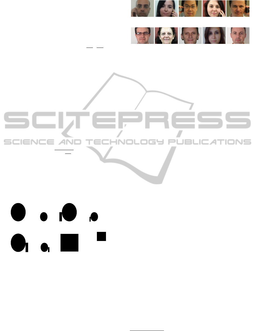
5 EXPERIMENTS
Experiments were performed on one set of images,
with 100 positive images (people with phone) and the
other 100 negative images (no phone). All images
are frontal. In Figure 3, sample images for the set of
images are exemplified.
SVM is used as classification technique to the sys-
tem. All tests have the same set of features and cross-
validation (Kohavi, 1995) is applied with 9 datasets
(a) (b) (c) (d) (e)
(a) (b) (c) (d) (e)
Figure 3: Sample images for the set of images. Positive
images are in first line. Negative images are in the second
line.
from the initial set. Genetic Algorithm or GA
3
(Gold-
berg, 1989) is used to find the parameters (nu, coe f 0,
degree, and γ for SVM) for maximum accuracy of
classification system.
GA is inspired by evolutionary biology, where the
evolution of a population of individuals (candidate so-
lutions) is simulated over several generations (itera-
tions) in search of the best individual. GA param-
eters, empirically defined, used on experiments: 20
individuals, 10, 000 generations, crossover 80%, mu-
tation 5%, and tournament as selector. The initial po-
pulation is randomly (random parameters) and subse-
quent generations are the evolution result. The classi-
fier is trained with parameters (genetic code) of each
individual using binary encoding of 116 bits. Finally,
the parameters of the individual that results in higher
accuracy (fitness scores) for the classifier are adopted.
GA was performed three times for each SVM kernel
defined in Section 3.1. The column “Parameters” of
Tables 1 shows the best parameters found for SVM.
SVM is tested on kernels: Linear, Polynomial,
RBF and Sigmoid (Section 3.1). The kernel that has a
highest average accuracy is the Polynomial, reaching
a rate of 91.57% with images of training set. Table 1
shows the results of the tests, parameters and accuracy
of each kernel.
The final tests are done with five videos
4
in real
environments with the same driver. All videos have
a variable frame rate. The average frame rate is 15
FPS. The resolution is 320 × 240 pixels for all. The
container format is 3GPP Media Release 4 for them.
The specific information about the videos are in Ta-
ble 2.
Some mistakes were observed in the frames in
preprocessing step (Section 4.1.1). The Table 3 shows
the problems encountered. In frames reported as “not
found” the driver cannot be found. The frames of the
column “wrong” are false positives, ie, the region de-
3
The library GALib version 2.4.7 is used (available in
http://lancet.mit.edu/ga).
4
See the videos on the link: http://www.youtube.com/
channel/UCvwDU26FDAv1xO000AKrX0w
VISAPP2014-InternationalConferenceonComputerVisionTheoryandApplications
414
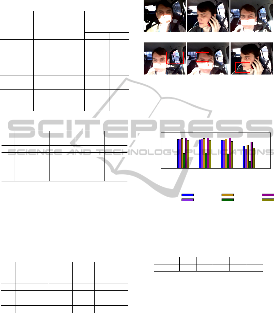
Table 1: Accuracy of SVM kernels.
Accuracy
(cross-
validation)
Kernel Parameters Average
σ
Linear
nu = 0.29
91.06% ±6.90
Polynomial
nu = 0.30
coe f 0 = 4761.00
degree = 0.25
γ = 5795.48
91.57% ±5.58
RBF
nu = 0.32
γ = 0.36
91.06% ±6.56
Sigmoid
nu = 0.23
coe f 0 = 1.82
γ = 22.52
89.06% ±8.79
Table 2: Information about the videos.
# Weather Time Duration Frames
V1 Overcast Noon 735 s 11,005
V2 Mainly sun Noon 1, 779 s 26, 686
V3 Sunny Noon 1,437 s 21,543
V4 Sunny Dawn 570 s 8,526
V5 Sunny Late af-
ternoon
630 s 9,431
clared as a driver is wrong. The preprocessing algo-
rithm was worst for Video 4 with rate error 24.20%.
Some frames with preprocessing problem are shown
in Figure 4. The best video for this step was Video
3 with rate error 3.31%. The rate error average for
all videos’ frames is 7.42%. The frames with prepro-
cessing errors were excluded from following experi-
ments.
Table 3: Error while searching for Driver (preprocessing).
# Not found Wrong Total
Frame rate
error
V1 237 273 510
4.63%
V2 675 974 1,649
6.18%
V3 356 358 714
3.31%
V4 1,280 783 2, 063
24.20%
V5 533 259 792
8.40%
Each frame of the video was segmented (Sec-
tion 4.1.2), extracted features (Section 4.1.3), and
classified by kernels. Figure 5 shows the results for
each combination of video/kernel and the last line
shows the average accuracy values for frames of all
videos. The polynomial kernel was the best on the
tests, it obtained an accuracy of 79.36%. For the next
experiment we opted for the polynomial kernel.
We performed time analysis splitting the videos in
(a) (b) (c)
(d) (e) (f)
Figure 4: Sample frames for preprocessing problem. The
frames in (a), (b), and (c) are examples for driver not found.
The frames in (d), (e), and (f) are examples for driver wrong,
and the red rectangle shows where the driver was found for
these images.
40
50
60
70
80
90
Linear
Polynomial
RBF
Sigmoid
%
Accuracy
Video 1
Video 2
Video 3
Video 4
Video 5
All frames
Figure 5: Accuracy for the kernels by frame.
periods of 3 seconds. The Table 4 shows the periods
quantity by video.
Table 4: Number of periods by video.
Videos V1 V2 V3 V4 V5
Periods 245 594 479 190 210
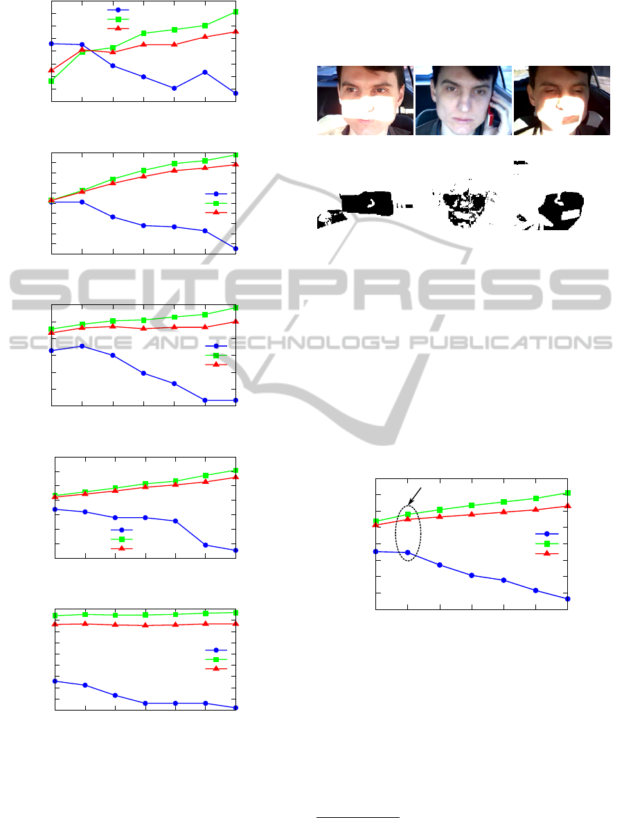
Detection of cell phone usage happens when the
period has the frames rate classified individually with
cell phone more or equal of a threshold. The threshold
values 60%, 65%, 70%, 75%, 80%, 85%, and 90%
were tested with the videos. The accuracy graphs
are shown in Figure 6. The columns “With phone”,
“No phone”, and “General” represent the accuracy
obtained for frame with cell phone, no cell phone, and
in general, respectively.
Figure 6(d) shows a larger distance between ac-
curacy “with phone” and “no phone” for the Videos
4 and 5. This difference is caused by problems with
preprocessing (Figure 4), and segmentation. The pre-
processing problems causes to decrease number of
frames analyzed in some periods, thus the classifica-
APatternRecognitionSystemforDetectingUseofMobilePhonesWhileDriving
415
82
84
86
88
90
92
94
96
98
60 65 70 75 80 85 90
Accuracy (%)
Threshold (%)
With phone
No phone
General
(a) V1
78
80
82
84
86
88
90
92
94
96
98
60 65 70 75 80 85 90
Accuracy (%)
Threshold (%)
With phone
No phone
General
(b) V2
65
70
75
80
85
90
95
60 65 70 75 80 85 90
Accuracy (%)
Threshold (%)
With phone
No phone
General
(c) V3
30
40
50
60
70
80
90
100
60 65 70 75 80 85 90
Accuracy (%)
Threshold (%)
With phone
No phone
General
(d) V4
10
20
30
40
50
60
70
80
90
100
60 65 70 75 80 85 90
Accuracy (%)
Threshold (%)
With phone
No phone
General
(e) V5
Figure 6: Accuracy for polynomial kernel by period and
video.
tion is impaired. Segmentation’s problems are caused
by the incidence of sunlight (close to twilight mainly)
on some regions of the driver’s face and the inner
parts of the vehicle. The sunlight changes the compo-
nents of pixels. Incorrect segmentation compromises
the feature extraction can lead to misclassification of
frames. Figure 7 exemplifies the segmentation pro-
blems.
(a) (b) (c)
(a) (b) (c)
Figure 7: Sample frames for segmentation problem. In first
line are examples for driver’s face. In second line are exam-
ples of segmentation.
Figure 8 presents the mean accuracy: “with
phone”, “no phone”, and in general, for videos at
each threshold. The accuracy of detecting cell phone
is greatest with thresholds 60% and 65%. The accu-
racy “no phone” for threshold 65% is better than 60%.
Thus, the threshold of 65% is more advantageous for
videos. This threshold results in accuracy for “with
phone” 77.33%, “no phone” 88.97%, and in general
of 87.43% at three videos.
60
65
70
75
80
85
90
95
100
60 65 70 75 80 85 90
Accuracy (%)
Threshold (%)
With phone
No phone
General
Figure 8: Graph of accuracy average (polynomial kernel)
by period for all videos of threshold by phone, No phone,
and General. The ellipse shows the best threshold.
5.1 Real Time System
The five videos
5
were simulated in real time on a com-
puter Intel i5 2.3GHz CPU, 6.0GB RAM and operat-
ing system Lubuntu 12.04. SVM/Polynomial classi-
fier was used, and training with the images set. The
5
See the videos with real time classifica-
tion on the link http://www.youtube.com/channel/
UCvwDU26FDAv1xO000AKrX0w
VISAPP2014-InternationalConferenceonComputerVisionTheoryandApplications
416
videos were used with a resolution of 320 × 240 pi-
xels.
The system uses parallel processing (multi-
thread), as follow one thread for image acquisition,
the frames are processed for four threads, and one
thread to display the result. Thus four frames can be
processed simultaneously. It shows able to process
up to 6.4 frames per second (FPS), however, to avoid
bottlenecks is adopted the rate 6 FPS for its execution.
The input image is changed to illustrate the result
of processing in the output of system. At left center
is added a vertical progress bar or historical percenta-
ge for frames “with phone” in the previous period (3
second). When the frames percentage is between 0%
and 40% green color is used to fill, the yellow color is
used between 40% and 65%, and red color above or
equal to 65%. Red indicates a risk situation. For real
situation should be started a beep. Figure 1 shows a
sequence of frames the system’s output.
Figure 9: The system’s output sequence sample in real time
with one frame for each second (15 seconds).
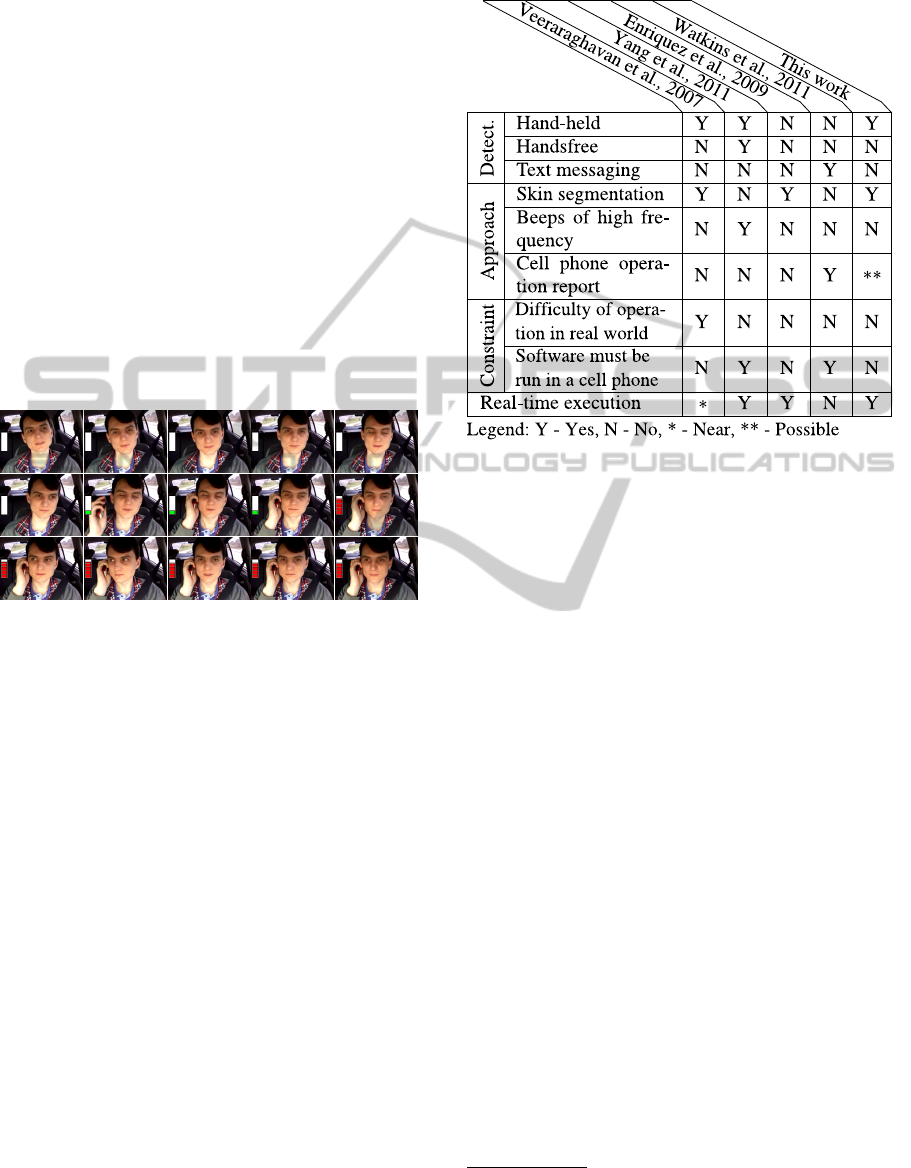
6 CONCLUSIONS
This paper presented an algorithm which allows ex-
traction features of an image to detect the use of cell
phones by drivers in a car. Very little literature on this
subject was observed (usually the focus is on drowsi-
ness detection or analysis of external objects or pedes-
trians). The Table 5 compare related works with this
work.
SVM and its kernels were tested as candidates to
solve the problem. The polynomial kernel (SVM) is
the most advantageous classification system with ave-
rage accuracy of 91.57% for set of images analyzed.
But, all the kernels tested have average accuracy sta-
tistically the same. GA found statistically similar pa-
rameters for all kernels.
Tests done on videos show that it is possible to
use the image datasets for training classifiers in real
situations. Periods of 3 seconds were correctly classi-
fied at 87.43% of cases. The segmentation algorithm
tends to fail when the sunlight falls (Videos 4 and 5)
at driver face and parts inside vehicle. This changes
Table 5: Table comparing related works and this work.
the components value for pixels of driver skin. Thus,
the pixels of skin for face and hand are different.
Enhanced cell phone use detection system is able
to find ways to works better when the sunlight falls
at the driver skin. Another improvement is to check
if the vehicle is moving and then execute the detec-
tion. An intelligent warning signal can be created,
i.e., more sensitive detection according to the speed
increases. One way is to join the OpenXC Platform
6
on solution to get the real speed among other data.
ACKNOWLEDGEMENTS
We thank CAPES/DS for the financial support to
Rafael Alceste Berri of Graduate Program in Ap-
plied Computing of Santa Catarina State University
(UDESC), and PROBIC/UDESC to Elaine Girardi of
Undergraduate program in Electrical Engineering.
REFERENCES
Balbinot, A. B., Zaro, M. A., and Timm, M. I. (2011).
Func¸
˜
oes psicol
´
ogicas e cognitivas presentes no ato
de dirigir e sua import
ˆ
ancia para os motoristas no
tr
ˆ
ansito. Ci
ˆ
encias e Cognic¸
˜
ao/Science and Cognition,
16(2).
Dadgostar, F. and Sarrafzadeh, A. (2006). An adaptive
real-time skin detector based on hue thresholding: A
6
It allows you to develop applications integrated with
the vehicle (available in http://openxcplatform.com)
APatternRecognitionSystemforDetectingUseofMobilePhonesWhileDriving
417

comparison on two motion tracking methods. Pattern
Recognition Letters, 27(12):1342–1352.
Drews, F. A., Pasupathi, M., and Strayer, D. L. (2008). Pas-
senger and cell phone conversations in simulated driv-
ing. Journal of Experimental Psychology: Applied,
14(4):392.
Enriquez, I. J. G., Bonilla, M. N. I., and Cortes, J. M. R.
(2009). Segmentacion de rostro por color de la piel
aplicado a deteccion de somnolencia en el conduc-
tor. Congreso Nacional de Ingenieria Electronica del
Golfo CONAGOLFO, pages 67–72.
Goldberg, D. E. (1989). Genetic Algorithms in Search, Op-
timization, and Machine Learning. Addison-Wesley
Professional, 1 edition.
Goodman, M., Benel, D., Lerner, N., Wierwille, W., Tije-
rina, L., and Bents, F. (1997). An investigation of the
safety implications of wireless communications in ve-
hicles. US Dept. of Transportation, National Highway
Transportation Safety Administration.
Hearst, M. A., Dumais, S. T., Osman, E., Platt, J., and
Sch
¨
olkopf, B. (1998). Support vector machines.
Intelligent Systems and their Applications, IEEE,
13(4):18–28.
Hu, M. K. (1962). Visual pattern recognition by moment
invariants. Information Theory, IRE Transactions on,
8(2):179–187.
Kohavi, R. (1995). A study of cross-validation and boot-
strap for accuracy estimation and model selection.
In International joint Conference on artificial intelli-
gence, volume 14, pages 1137–1145. Lawrence Erl-
baum Associates Ltd.
NHTSA (2011). Driver electronic device use in 2010. Traf-
fic Safety Facts - December 2011, pages 1–8.
Peissner, M., Doebler, V., and Metze, F. (2011). Can voice
interaction help reducing the level of distraction and
prevent accidents?
Regan, M. A., Lee, J. D., and Young, K. L. (2008). Driver
distraction: Theory, effects, and mitigation. CRC.
Smith, J. R. and Chang, S. F. (1996). Tools and techniques
for color image retrieval. In SPIE proceedings, vol-
ume 2670, pages 1630–1639.
Stanimirova, I.,
¨
Ust
¨
un, B., Cajka, T., Riddelova, K., Ha-
jslova, J., Buydens, L., and Walczak, B. (2010). Trac-
ing the geographical origin of honeys based on volatile
compounds profiles assessment using pattern recogni-
tion techniques. Food Chemistry, 118(1):171–176.
Strayer, D. L., Cooper, J. M., Turrill, J., Coleman, J.,
Medeiros-Ward, N., and Biondi, F. (2013). Measuring
cognitive distraction in the automobile. AAA Founda-
tion for Traffic Safety - June 2013, pages 1–34.
Strayer, D. L., Watson, J. M., and Drews, F. A. (2011).
2 cognitive distraction while multitasking in the au-
tomobile. Psychology of Learning and Motivation-
Advances in Research and Theory, 54:29.
Vapnik, V. (1995). The nature of statistical learning theory.
Springer-Verlag, New York.
Veeraraghavan, H., Bird, N., Atev, S., and Papanikolopou-
los, N. (2007). Classifiers for driver activity monito-
ring. Transportation Research Part C: Emerging Tech-
nologies, 15(1):51–67.
Viola, P. and Jones, M. (2001). Robust real-time object
detection. International Journal of Computer Vision,
57(2):137–154.
Wang, L. (2005). Support Vector Machines: theory and
applications, volume 177. Springer, Berlin, Germany.
Watkins, M. L., Amaya, I. A., Keller, P. E., Hughes, M. A.,
and Beck, E. D. (2011). Autonomous detection of dis-
tracted driving by cell phone. In Intelligent Trans-
portation Systems (ITSC), 2011 14th International
IEEE Conference on, pages 1960–1965. IEEE.
Yang, J., Sidhom, S., Chandrasekaran, G., Vu, T., Liu, H.,
Cecan, N., Chen, Y., Gruteser, M., and Martin, R. P.
(2011). Detecting driver phone use leveraging car
speakers. In Proceedings of the 17th annual interna-
tional conference on Mobile computing and network-
ing, pages 97–108. ACM.
VISAPP2014-InternationalConferenceonComputerVisionTheoryandApplications
418
