Swapping-based Annealed Particle Filter with Occlusion Handling

for 3D Human Body Tracking

Xuan Son Nguyen

INRIA, Loria, Campus Scientiﬁque, Vandœuvre-L

es-Nancy, France

Keywords:

Particle Filter, Human Body Tracking, Bayesian Network.

Abstract:

In this paper, we propose a new approach for 3D human body tracking. We ﬁrst extend the idea of Swapping-

based Partitioned Sampling (SBPS), which was introduced by Dubuisson et al. for solving the articulated

object tracking problem in high dimensional state spaces. This extension aims to deal with self-occlusion and

constraints between parts of the human body, which are not taken into account in SBPS. We prove that, under

the same assumptions required by SBPS, the posterior distribution are correctly estimated in our framework.

We then introduce a new approach for 3D human body tracking, based on this new framework and Annealed

Particle Filter (APF). Experiments with multi-camera walking sequences from the HumanEva I dataset show

the efﬁciency of the proposed approach in terms of both accuracy and computation time.

1 INTRODUCTION

Tracking the human body with accuracy and within a

reasonable time is challenging due to the high com-

plexity of the problem to solve. Various approaches

have been proposed for this problem. One class of

approaches is known as optimization-based methods

(Deutscher and Reid, 2005; Zhang et al., 2010). Typ-

ically, these methods are based on the optimization of

an objective function corresponding to the matching

function between the model and the observed image

features.

Another way of reducing the dimensionality of

the conﬁguration space is to use decomposition meth-

ods within the particle ﬁlter framework (MacCormick

and Isard, 2000; Rose et al., 2008). Particle Filter

(PF) (Gordon et al., 1993) has been shown to be an ef-

fective method for solving visual tracking problems.

This is due to its ability to deal with non-linear, non-

Gaussian and multimodal distributions encountered in

such problems. The key idea behind decomposition

methods is similar: decompose the state space of the

target object into a set of subspaces where particle

ﬁlter can be applied. Since the dimension of these

subspaces is smaller than that of the original state

space, sampling in these subspaces will be more ef-

ﬁcient than sampling in the original space and there-

fore, fewer particles are needed to achieve a good per-

formance. Recently, a decomposition approach called

Swapping-based Partitioned Sampling (SBPS), which

is based on the state-of-the-art algorithm Partitioned

Sampling (PS) (MacCormick and Isard, 2000) for

tracking in high dimensional state spaces, has been in-

troduced in (Dubuisson et al., 2011; Dubuisson et al.,

2013). Under some assumptions, SBPS is guaranteed

to produce a correct estimation of the posterior dis-

tribution. However, one of the important assumptions

required by SBPS is that no self-occlusion occurs dur-

ing tracking. This assumption is often violated in real-

world problems, and the posterior distribution can be

poorly approximated by SBPS in such cases. An-

other disadvantage of SBPS is that it does not take

into account constraints between different parts of the

articulated object, which have been shown to be very

important in human tracking (Sigal et al., 2010). To

address these problems, we ﬁrst introduce an exten-

sion of SBPS, which is more ﬂexible than SBPS and

allows us to better estimate the posterior distribution

when self-occlusion is present. We then introduce a

new approach for 3D human body tracking, which is

a combination of the new framework and Annealed

Particle Filter (APF) (Deutscher and Reid, 2005).

The paper is organized as follows. In Section 2,

we give a brief introduction to PF, PS and SBPS. Sec-

tion 3 presents the proposed approach. Section 4 re-

ports the results of our experimental evaluation. Fi-

nally, Section 5 offers some conclusions and ideas for

future work.

576

Nguyen X..

Swapping-based Annealed Particle Filter with Occlusion Handling for 3D Human Body Tracking.

DOI: 10.5220/0004686905760583

In Proceedings of the 9th International Conference on Computer Vision Theory and Applications (VISAPP-2014), pages 576-583

ISBN: 978-989-758-009-3

 2014 SCITEPRESS (Science and Technology Publications, Lda.)

2 RELATED WORK

2.1 Particle Filter

In this paper, human tracking consists of estimat-

ing a state sequence {x

}

t=1,...,T

, whose evolution is

given by equation x

= f

t−1

, n

), from observations

}

t=1,...,T

related to the states by y

= h

, n

Usually, f

and h

are nonlinear functions, and n

and n

are i.i.d. noise sequences. From a proba-

bilistic viewpoint, it amounts to estimate, for any t,

p(x

1:t

) where x

1:t

denotes the tuple (x

, . . . , x

The PF framework (Gordon et al., 1993) approxi-

mates the posterior densities using weighted samples

(i)

, w

(i)

}, i = 1, . . . , N, where each x

(i)

is a possible

realization of state x

called a particle. In its predic-

tion step, PF propagates the particle set {x

(i)

t−1

, w

(i)

t−1

}

using a proposal function q(x

(i)

1:t−1

) which may

differ from p(x

(i)

t-1

) (but, for simplicity, we will as-

sume they do not); in its correction step, PF weights

the particles using a likelihood function, so that

(i)

∝ w

(i)

t−1

p(y

(i)

)

p(x

(i)

t−1

)

q(x

(i)

1:t−1

)

, with

∑

i=1

(i)

= 1.

The particles can then be resampled: those with the

highest weights are duplicated while the others are

eliminated. The estimation of the posterior density

p(x

1:t

) is then given by

∑

i=1

(i)

), where

(i)

are Dirac masses centered on particles x

(i)

2.2 Partitioned Sampling and

Swapping-based Partitioned

Sampling

Partitioned Sampling (PS) has been introduced by

MacCormick (MacCormick and Isard, 2000). PS’s

key idea is to exploit some natural decomposition

of the system dynamics w.r.t. subspaces of the state

space in order to apply PF only on those subspaces.

This leads to a signiﬁcant reduction in the number of

particles required for tracking. So, assume that state

space X and observation space Y can be partitioned

as X = X

× ··· × X

and Y = Y

× ··· × Y

re-

spectively. For instance, a system representing a hand

could be deﬁned as X

hand

= X

palm

×X

thumb

×X

index

middle

× X

ring

× X

little

. Assume in addition that the

dynamics of the system follows this decomposition,

i.e., that:

t−1

, n

) = f

◦ f

P−1

◦ ··· ◦ f

◦ f

t−1

), (1)

where ◦ is the usual function composition operator

and where each function f

: X 7→ X modiﬁes the par-

4 7

1310

t−1

time t − 1 time t

t−1

Figure 1: Full body tracking.

ticles’ states only on subspace X

i 1

In PS, one assumes that the global image likeli-

hood can be factorized as product of local likelihoods:

p(y

) =

∏

i=1

), (2)

where y

and x

are the projections of y

and x

on Y

and X

respectively.

Swapping-based Partitioned Sampling (SBPS) has

been introduced in (Dubuisson et al., 2011). It ex-

ploits conditional independences encoded in Dynamic

Bayesian Networks (DBNs) (Murphy, 2002) to im-

prove the tracking accuracy and reduce the computa-

tional cost of PS. Figure 1 show an example of hu-

man body tracking and a DBN used by SBPS for

modeling this problem, where x

, k = 1, ...15 repre-

sent the parts of the human body. Denote pa(x

) and

) the parent of node x

in all time instants and in

time instant t, respectively. The assumptions required

by SBPS is that the proposal transition function of a

given part x

at time t depends only on that part in

time t − 1 (and possibly on other parts in time t) and

the observations depend only on their corresponding

state. The set {1, . . . , P} of parts of the target ob-

jects can be partitioned into some sets {P

, . . . , P

}

such that those parts in each P

are all independent

conditionally to ∪

h< j

. For instance, in Figure 1,

P = 15 and K = 5, P

= {1} corresponds to the pelvis,

= {2, 3, 6} to the torso, the right and left thighs,

= {4, 7, 9, 12, 15} to the right and left calves, the

right and left upper arms, the head, P

= {5, 8, 10, 13}

to the right and left foots, the right and left lower

arms, P

= {11, 14} to the right and left hands. At

Note that, in (MacCormick and Isard, 2000), func-

tions f

are more general since they can modify states on

× ··· × X

. However, in practice, particles are often

propagated only one X

at a time.

Swapping-basedAnnealedParticleFilterwithOcclusionHandlingfor3DHumanBodyTracking

577

∼

∗ f



p(x

t−1

1:t−1

)

p(x

1:t

)

∗ f

B(4)

∗ f

B(7)

∗ f

B(10)

∗ f

B(13)

×p

Figure 2: New diagram for SBPS.

the jth stage, SBPS performs the prediction/correction

steps for the parts in P

in parallel instead of part after

part as in PS. This enables to produce better parti-

cles by swapping their subparts. This is achieved by

an operation called swapping or permutation, which

guarantees that the target distribution is correctly es-

timated. More precisely, whenever two particles are

such that they have the same states on some nodes

), then swapping their states on x

and its de-

scendants cannot alter the density estimated by the

particle set. For instance, on Figure 1, if two particles

have the same value for node pa

), their values on

node x

, x

and x

can be safely swapped. The set of

subparts to permute similarly to x

in called a swap-

ping set. In addition, subpart permutation between

two particles can only be performed if they have the

same states on some nodes pa

), which leads to

the deﬁnition of what is admissible permutation. In

SBPS, the deﬁnitions of swapping set and admissible

permutation guarantee that densities are correctly es-

timated.

The soundness of SBPS can be justiﬁed by d-

separation analysis on DBNs (see (Dubuisson et al.,

2013)).

3 PROPOSED APPROACH

SBPS is based on an important assumption that the

global image likelihood can be expressed as a prod-

uct of individual local likelihoods. The likelihood

for each part of the target object is then evaluated in-

dependently of other parts without taking into con-

sideration self-occlusion. When self-occlusions are

present however, this assumption is violated and the

product of local likelihoods gives a poor approxima-

tion to the global likelihood. As a result, SBPS tracker

does not give good performances when tracking un-

der self-occlusions. To cope with this problem, we

propose a new diagram for SBPS. We ﬁrst introduce a

theoretical framework for this diagram in the next sec-

tion. Then, in section 3.2, we propose a new approach

for 3D human body tracking, based on this diagram.

3.1 Theoretical Framework

For computational reason, we will assume from this

point on that, within each time slice, the DBN struc-

ture is a directed tree.

For any u, u = 1, . . . , P, denote T (u) the set of

indices of nodes in the subtree whose root is x

(the indice of node x

for any t is u). Denote P

any subset of {1, . . . , P} such that: if u

∈ P

then

∈ P

where x

= pa

). For any j ≥ 2, as-

sume that P

, . . . , P

j−1

have been deﬁned. Let S

be any subset of the set of nodes that have not

been selected in any set P

, . . . , P

j−1

and any node

in S

is some child node of a node in P

∪ . . . ∪

j−1

: S

⊆ {u ∈ {1, . . . , P}\ ∪

j−1

h=1

: pa

) ⊆

j−1

h=1

v∈P

}}. For all u ∈ S

, denote B(u) any

subset of T (u) such that: if u

6= u and u

∈ B(u) then

∈ B(u) where x

= pa

). Then P

is deﬁned

as: P

u∈S

B(u). In order to determine interest-

ing permutations, denote F

, . . . , F

a partition of P

such that any F

, h = 1, . . . , n

is a union of some sets

B(u), u ∈ S

. We call F

, . . . , F

an interesting parti-

tion of P

As an example, consider the human tracking prob-

lem in Figure 1. Here we have P = {1, . . . , 15}.

Assume that P

= {1, 2, 3, 6, 9, 12, 15} and now we

want to deﬁne P

. We can deﬁne S

= {4, 7, 10, 13}

since any node in S

is a child node of a node

in P

. Then we can deﬁne the following sets:

B(4) = {4, 5}, B(7) = {7, 8}, B(10) = {10, 11},

B(13) = {13, 14} and hence P

= B(4) ∪ B(7) ∪

B(10) ∪ B(13) = {4, 5, 7, 8, 10, 11, 13, 14}. We par-

tition P

into F

, F

where: F

= B(4) ∪ B(7),

= B(10) ∪ B(13). In this case, a new dia-

gram for SBPS can be described in Figure 2, where

∗ f

, ∗ f

B(4)

, ∗ f

B(7)

, ∗ f

B(10)

, ∗ f

B(13)

refer to propaga-

tion of nodes in P

, B(4), B(7), B(10), B(13) in topo-

logical orders, respectively. ×p

, ×p

re-

fer to the correction step where particle weights are

multiplied by p

, p

, respectively. 

refers

to the particle subpart swappings, where we permute

the substates in F

among particles having the same

states for x

∪ x

, and where we permute the sub-

states in F

among particles having the same states

for x

∪ x

. In general case, the swapping set and

admissible permutation are deﬁned as follows:

Deﬁnition 1. Let F be a set in an interesting partition

of P

. Let u

, . . . , u

∈ S

are such that F =

i=1

B(u

The set x

i=1

B(u

)

i=1

(T (u

)\B(u

))

t−1

is called a swap-

ping set. A permutation σ : {1, . . . , N} 7→ {1, . . . , N}

VISAPP2014-InternationalConferenceonComputerVisionTheoryandApplications

578

is said to be admissible if and only if x

(i),h

= x

(σ(i)),h

for all i ∈ {1, . . . , N} and for all nodes x

∈ ∪

s=1

∪

i=1

The correctness of the diagram in Figure 2 follows

from Proposition 1 (see Appendix for the proof).

Proposition 1. Under the same assumptions required

by SBPS, the set of particles resulting from the dia-

gram of Figure 2 represents probability distribution

p(x

1:t

It should be noted that the application of our the-

oretical framework is not limited for DBNs whose

structures are directed trees. However, since the

swapping sets and admissible permutations can be

identiﬁed more easily in directed tree cases, an efﬁ-

cient implementation of the tracking algorithm can be

obtained for these cases.

The main advantage of the diagram in Figure 2

compared to that of SBPS is that self-occlusion or

constraints between parts of the articulated object can

be efﬁciently taken into account. Let us consider the

case of self-occlusion. Actually, there are two inter-

esting cases where the diagram in Figure 2 are partic-

ularly useful when dealing with self-occlusion. The

ﬁrst case is when we do not have observation for each

part but only for a group of parts. In this case, the

evaluation of the likelihood for each body part, as re-

quired by SBPS, often gives poor approximations, re-

sulting in bad tracking results due to poor approxima-

tions of the global likelihood in Equation 2. Now, sup-

posing that P

, F

and F

are groups of parts where

we can obtain good observation for each group. In

other words, we can obtain good approximations for

, p

and p

. Then, the global likelihood can be

better approximated as follows:

p(y

) = p

× p

The second case where the diagram in Figure 2

is useful for dealing with self-occlusion is when

the observation on some parts (guiding parts) pro-

vides search constraints for some other parts (primary

parts) that are estimated just before the guiding parts

when tracking the object. In this case, it could be

more efﬁcient to combine the guiding parts and the

primary parts into some set F (for instance, F

or F

in the diagram of Figure 2) in order to improve the es-

timates for the primary parts and thus for the guiding

parts.

The diagram in Figure 2 also allows us to apply

some types of hard prior which SBPS ﬁnds it difﬁcult

to deal with. These hard priors eliminate any particle

that violates some constraint between parts of the ar-

ticulated object, thus reduce the search space. Let us

Figure 3: Human body model.

consider the case when one wants to impose a pair-

wise constraint between two parts belonging to two

different branches of the tree representing the articu-

lated object. In the case their parent parts are poorly

estimated, then at the prediction step of these parts, it

could happen that the process of generating new parti-

cles for them must be repeated a lot of times to obtain

the required number of particles satisfying the con-

straint. This process may increase the computational

time by unpredictable amounts. In such situation, one

might want to backtrack and regenerate new conﬁgu-

rations for their parent parts. Such a task can not be

achieved in SBPS since any part in SBPS is always

processed after its parent parts and before its child

parts. In the diagram of Figure 2, the capability of

processing in parallel a group of parts belonging to

the same branch of the tree enables an efﬁcient way

of dealing with some types of hard prior.

3.2 Our Approach for Human Tracking

3.2.1 Body Model and Likelihood Model

We use the human body model in (Sigal et al., 2010),

which is shown in Figure 3. The model consists of 15

parts where body parts are connected by joints. Track-

ing consists of estimating at each time instant a vector

of 34 parameters comprising the global position and

orientation of the pelvis and the relative joint angles

between neighboring limbs.

The likelihood model consists of a edge-based

part and a silhouette-based part, which is commonly-

used likelihood model for human body tracking. We

refer the reader to (Deutscher and Reid, 2005; Sigal

et al., 2010). Our human body tracking problem can

be modeled by the DBN in Figure 1.

3.2.2 Self-occlusion Handling

Like SBPS, our idea is to partition P into some sub-

sets. Body parts in these subsets are estimated se-

Swapping-basedAnnealedParticleFilterwithOcclusionHandlingfor3DHumanBodyTracking

579

quentially, while within each subset, body parts or

groups of body parts are processed in parallel. Here,

we partition P into 2 subsets: P

= {1, 2}, P

{3, 4, 5, 6, 7, 8, 9, 10, 11, 12, 13, 14, 15}. P

is then par-

titioned into F

and F

where: F

= {3, 4, 5, 6, 7, 8},

= {9, 10, 11, 12, 13, 14, 15}. It is easy to see that

the sets P

, P

, F

follow the deﬁnitions in sec-

tion 3.1. This partition is motivated by the fact that

during normal human activities like walking or jog-

ging, the left and right legs often occlude each other

and should be processed in parallel. Also, the left and

right arms often occlude each other and should be pro-

cessed in parallel.

3.2.3 Dealing with Hard Prior

In (Sigal et al., 2010), to reduce the search space, a

hard prior is applied that eliminates any particle that

corresponds to implausible body poses such as hav-

ing angles exceeding anatomical joint limits or inter-

penetrating limbs. This has been shown to improve

signiﬁcantly the performance of the tracking algo-

rithms. By partitioning P into P

, P

, such a hard

prior can naturally be applied in our approach. More

precisely, when processing P

, we can test for inter-

sections between the left and right calves, since P

contains all parameters describing the conﬁguration

of the legs. Similarly, test for intersections between

the lower arms and the torso can be performed when

processing P

, since P

contains all parameters de-

scribing the conﬁguration of the arms, and at the time

we process P

, the conﬁguration of the torso has been

previously determined in P

. Finally, constraints on

anatomical joint limits can be imposed at any time we

process P

and P

3.2.4 Algorithm

Our approach is based on the approach in (Dubuisson

and Gonzales, 2012) (we call it SB-PSAPF), which

combines the idea of SBPS and Partitioned Sampling

Annealed Particle Filter (PSAPF) (Bandouch et al.,

2008). In this approach, an annealing run consists of

parallel propagation/correction steps for a set of parts,

followed by a swapping operation over this set, and ﬁ-

nally by a resampling. By testing on a human tracking

problem, this approach has been shown to be effec-

tive. However, the tracking conditions in this prob-

lem is quite simple, where no cluttered background is

present and no self-occlusion occurs during tracking.

Actually, these conditions are necessary for the as-

sumptions in Equation 2 to be satisﬁed. In real world

problems, when these assumptions do not hold, the

global likelihood might be poorly approximated, re-

sulting in poor tracking results. Furthermore, the use

of the swapping operation in multiple layers frame-

work, as proposed in SB-PSAPF, creates another is-

sue. Although this operation generates more particles

near the modes of the target distribution, it creates the

well-known sample impoverishment problem. The

reason is that after applying it on a particle set, it in-

creases the differences between particle weights. Af-

ter resampling, only particles with highest weight are

multiplied, while the remaining particles (those with

medium weights and low weights) have little chance

to survive. In SB-PSAPF, the sample impoverishment

problem is worst since at each layer, the swapping op-

eration is performed once and the diversity of the par-

ticle set decreases as the number of layers increases.

Another drawback of SB-PSAPF is that it esti-

mates the ﬁrst set of body parts, without taking into

account their relation with the remaining body parts.

In our case, it estimates the pelvis and the torso with-

out looking at the head and the limbs. In practice,

however, some body parts, such as and the legs and

the head often provide important constraints for ﬁnd-

ing the pelvis and the torso, and therefore it is not

always possible to localize the pelvis and the torso

separately from other body parts. When the pelvis

and the torso are poorly estimated, this affects the es-

timates of the head and the limbs and the performance

of the tracking algorithm degrades.

To address the problems discussed above, we pro-

pose a two-stages tracking strategy, where in the ﬁrst

stage, human body parts are tracked using APF and

in the second stage, the estimates of the head and

the limbs are reﬁned using SB-PSAPF, except that we

omit the optimization step for the pelvis and the torso.

At each time instant, an annealing run in the second

stage of our algorithm consists of the following steps:

Step 1: The particle set is resampled

Step 2: The parts in P

are propagated using their

dynamic functions. The hard prior, which is discussed

in this section, is applied. This step is repeated until

obtaining the required number of particles.

Step 3: For each particle, the likelihoods of the

substates corresponding to the body parts in F

and

are evaluated (for the sake of convenience, we call

them the likelihoods of F

and F

, respectively). For

, the legs of the human body model are ﬁrst pro-

jected into edge images and silhouette images and

then the likelihood of F

is computed as in (Sigal

et al., 2010). In this way, one evaluation of the like-

lihood function in this step requires less computation

time than that in APF, since only body parts related to

the evaluation are projected.

Step 4: The substates corresponding to the body

parts in F

can be permuted among particles having

the same value for the pelvis. Also, the substates cor-

VISAPP2014-InternationalConferenceonComputerVisionTheoryandApplications

580

Table 1: Tracking errors and standard deviations (mm)

of APF, SB-PSAPF and our approach from tracking the

walking sequences of S1, S2, S3 with 590, 438 and 448

frames, respectively. The processing times shown below

each method are computed for one frame and one camera.

Sequence S1 S2 S3

SB-PSAPF 242±40 230±34 285±45

(12s)

SB-PSAPF2 220±32 211±25 265±35

(11s)

APF 125±37 105±20 199±41

(6s)

Our approach 120±26 95±12 182±30

(4s)

responding to the body parts in F

can be permuted

among particles having the same value for the torso.

The new weight of each particle is computed by tak-

ing the product of the likelihoods of F

and F

. In

order to generate a better particle set, at each step, the

particle with highest weight resulting from all pos-

sible permutations is constructed and added into the

new particle set. This particle is then eliminated from

the current particle set and the process is repeated.

Step 5: The particle weights are annealed as

in (Deutscher and Reid, 2005) so that about a half of

the particle set will survive the next resampling step.

4 EXPERIMENTAL RESULTS

In this section, we quantitatively compare our ap-

proach with APF, SB-PSAPF and SB-PSAPF2. For

SB-PSAPF, we estimate the pelvis and the torso at

the ﬁrst stage, the head, the left and right upper arms,

the left and right thighs at the second stage, the left

and right lower arms, the left and right calves at the

third stage, and ﬁnally the left and right foots, the left

and right hands at the forth stage. SB-PSAPF2 is a

variant of SB-PSAPF where we use the same parti-

tion as our approach. For both SB-PSAPF and SB-

PSAPF2, the same hard prior used in our approach is

applied to improve their performance. The compari-

son between SB-PSAPF and SB-PSAPF2 will show

the interest of the diagram in Figure 2 when dealing

with self-occlusion. In order to ensure a fair compari-

son, we use the HumanEva dataset (Sigal et al., 2010),

which provides an implementation of APF. We im-

plement our algorithm, SB-PSAPF and SB-PSAPF2

within their framework, while keeping the remaining

codes unchanged. We use the error measure in (Sigal

et al., 2010), which averages the Euclidean distance

between 15 markers on the true pose and the corre-

sponding points computed from the estimated pose.

The likelihood model is constructed from edges and

silhouettes (Sigal et al., 2010). The image sequences

from 5 camera views: C1, C2, C3, BW1, BW2 are

used. First-order temporal dynamics are used where

the sampling covariance is learnt from all training

data in the dataset.

For our approach, we use 400 evaluations of the

likelihood function per frame, which is equal to 5 lay-

ers with 50 particles per layer for the ﬁrst stage, and

3 layers with 50 particles per layer for the second

stage. For APF, we use 500 evaluations of the like-

lihood function per frame, which is equal to 5 layers

with 100 particles per layer. For SB-PSAPF and SB-

PSAPF2, we use 1000 evaluations of the likelihood

function per frame, which is equal to 5 layers with 50

particles per layer in 4 stages for SB-PSAPF, and 5

layers with 100 particles per layer in both stages for

SB-PSAPF2.

We present in this section the tracking results for

the walking sequences of S1, S2 and S3. Table 1

shows the tracking errors and standard deviations of

4 approaches from tracking S1, S2 and S3. As can

be observed, SB-PSAPF has the worst performance.

Due to self-occlusions between the legs and between

the torso and the arms, the evaluation of the likeli-

hood for each body part, as required by SB-PSAPF,

gives poor approximations. This leads to poor per-

formances of SB-PSAPF. By taking into account self-

occlusion, SB-PSAPF2 improves the performance of

SB-PSAPF. For 3 sequences, our approach achieves

better performances than the other approaches in term

of tracking error, standard deviation and computation

time. We can observe that the tracking errors obtained

from tracking S3 are higher than those obtained from

tracking S1 and S2. This is due to larger movements

of the legs of S3 compared to S1 and S2. We can also

observe that the difference between the tracking errors

of our approach and APF from tracking S3 are larger

that those obtained from tracking S1 and S2. This re-

sult suggests that our approach is robust in tracking

people with strong motions.

Figure 4 shows some frames from tracking S3, us-

ing APF and our approach. At frame 100, our ap-

proach fails to track the right leg, as APF does (see

the 2nd column). However, at the next frames, our

approach can recover from tracking failure and tracks

the legs quite well, while APF fails to track one of

the two legs correctly. This highlights the effective-

ness of the second stage of our approach in reﬁning

the estimate for the limbs. Figure 5 shows the track-

Swapping-basedAnnealedParticleFilterwithOcclusionHandlingfor3DHumanBodyTracking

581

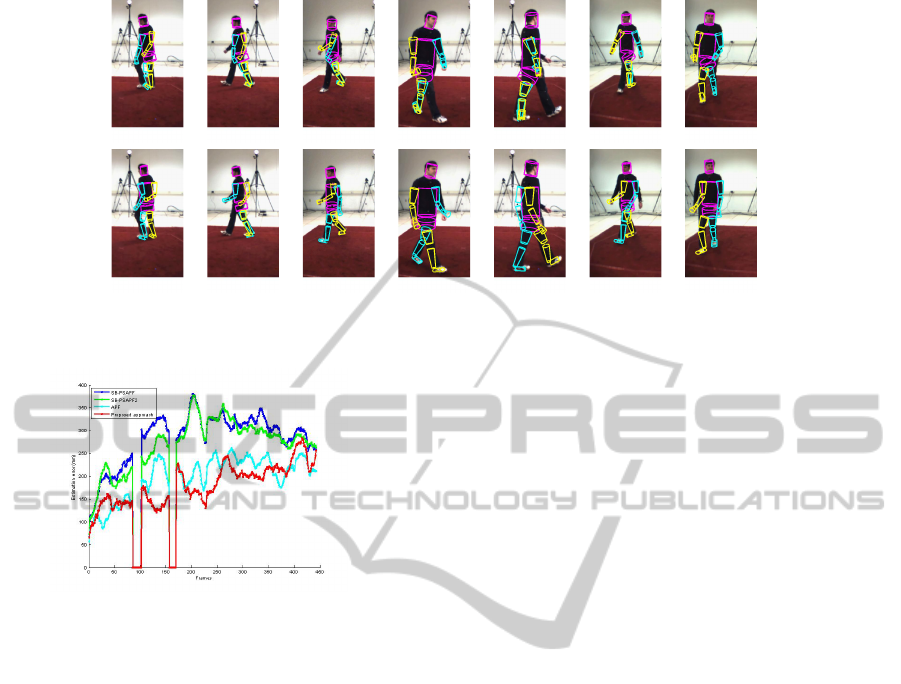
Figure 4: Tracking results of the sequence S3 walking for frames 51,100, 240 303,340, 382. APF (1th row), our approach

(2nd row). The images in the ﬁrst 5 frames are obtained from one view and those in the last 2 frames are obtained from

another view to better visualize the tracking results for the legs of 2 approaches.

Figure 5: Tracking errors (mean over 10 runs) of SB-

PSAPF, SB-PSAPF2, APF and our approach for the walk-

ing sequence of S3.

ing error curves of 4 approaches from tracking S3.

There are two intervals where we can not obtain the

groundtruth, due to bad data. Hence, we set the track-

ing errors of 4 approaches to zero for these intervals.

As can be observed, our approach is clearly better

than the other approaches at most of the frames.

5 CONCLUSIONS

We have presented a new particle ﬁlter based ap-

proach for 3D human body tracking. Our approach

consists of 2 stages. At the ﬁrst stage, the human

body is tracked using Annealed Particle Filter. Then,

the limbs are reﬁned using another stage, where more

particles near the modes of the likelihood function are

generated by swapping the substates of the particles.

This second stage is also based on the framework of

Annealed Particle Filter. Our quantitative evaluation

on real sequences has shown the robustness of the pro-

posed approach. It should be noted that our theoreti-

cal framework proposed in section 3.1, can be applied

not only for tracking articulated objects but also for

tracking multiple objects interacting with each oth-

ers. Here, the advantage compared to SBPS is that

occlusions and constraints between objects can be ef-

fectively taken into account. Although our approach

improves the estimate of the limbs thanks to its sec-

ond stages, the obtained tracking results are not satis-

factory due to self-occlusion. Our current work focus

on developing more efﬁcient methods for dealing with

these problems within our framework.

REFERENCES

Bandouch, J., Engstler, F., and Beetz, M. (2008). Evalua-

tion of Hierarchical Sampling Strategies in 3D Human

Pose Estimation. In BMVC, pages 925–934.

Deutscher, J. and Reid, I. (2005). Articulated body motion

capture by stochastic search. International Journal of

Computer Vision, 61(2):185–205.

Dubuisson, S. and Gonzales, C. (2012). An optimized dbn-

based mode-focussing particle ﬁlter. In Proceedings

of the 2012 IEEE Conference on Computer Vision and

Pattern Recognition (CVPR). IEEE Computer Society.

Dubuisson, S., Gonzales, C., and Nguyen, X. S. (2011).

Swapping-based partitioned sampling for better com-

plex density estimation: Application to articulated ob-

ject tracking. In International Conference on Scalable

Uncertainty Management, pages 525–538.

Dubuisson, S., Gonzales, C., and Nguyen, X. S. (2013).

Sub-sample swapping for sequential monte carlo ap-

proximation of high-dimensional densities in the con-

text of complex object tracking. International Journal

of Approximate Reasoning, 54(7):934 – 953.

Gordon, N., Salmond, D. J., and Smith, A. (1993). Novel

approach to nonlinear/non-Gaussian Bayesian state

estimation. IEE Proceedings of Radar and Signal Pro-

cessing.

MacCormick, J. and Isard, M. (2000). Partitioned sampling,

articulated objects, and interface-quality hand track-

ing. In ECCV, pages 3–19.

Murphy, K. P. (2002). Dynamic Bayesian Networks : Rep-

VISAPP2014-InternationalConferenceonComputerVisionTheoryandApplications

582

resentation, Inference and Learning. PhD thesis, Uni-

versity of California, Berkeley.

Rose, C., Saboune, J., and Charpillet, F. (2008). Reducing

particle ﬁltering complexity for 3D motion capture us-

ing dynamic Bayesian networks. ICAI, pages 1396–

1401.

Sigal, L., Balan, A., and Black, M. (2010). Humaneva: Syn-

chronized video and motion capture dataset and base-

line algorithm for evaluation of articulated humanmo-

tion. International Journal of Computer Vision, 87(1-

2):4–27.

Zhang, X., Hu, W., Wang, X., Kong, Y., Xie, N., Wang,

H., Ling, H., and Maybank, S. (2010). A swarm in-

telligence based searching strategy for articulated 3D

human body tracking. In CVPR, pages 45–50.

APPENDIX

Proposition 1. We denote by Q

= ∪

h=1

and R

∪

h= j+1

the set of parts already processed after the

jth step of the diagram in Figure 2 (the jth step

consists of processing parts in P

) and those still to

be processed, respectively. By convention, we set

= R

0. We shall show that 1) after the prop-

agations of parts in P

(prediction step), the particle

set represents the density p(x

, x

t−1

1:t−1

, y

j−1

);

2) after the corrections of parts in P

, the particle set

represents the density p(x

, x

t−1

1:t−1

, y

); 3) af-

ter the swapping of parts in P

, the particle set rep-

resents the density p(x

, x

t−1

1:t−1

, y

); Since the

resampling step does not alter the distribution repre-

sented by the particle set, at the last step (Kth step) of

the diagram in Figure 2, the particle set represents the

density p(x

, x

t−1

1:t−1

, y

) = p(x

1:t−1

, y

) =

p(x

1:t

We prove 1), 2), 3) by introduction on j. Assume

that after the (j-1)th step, the particle set represents the

density p(x

j−1

, x

j−1

t−1

1:t−1

, y

j−1

). For the proof of

1) and 2), we refer the reader to (Dubuisson et al.,

2013). We now prove 3). Let F be a set in an inter-

esting partition of P

and let u

, . . . , u

∈ S

are such

that F =

i=1

B(u

). Denote x

= x

∪

i=1

B(u

)

, x

t−1

∪

i=1

(T (u

)\B(u

))

t−1

, x

= ∪

i=1

), x

= x

\(C∪A)

t−1

= x

t−1

\ x

t−1

. From 2), after the corrections of

parts in P

, the particle set estimates the distribution

p(x

, x

t−1

1:t−1

, y

). We have:

p(x

, x

t−1

1:t−1

, y

) ∝ p(x

, x

t−1

, y

1:t−1

, y

)

= p(x

C∪A∪V

, x

D∪W

t−1

, y

C∪A∪V

1:t

, y

D∪W

1:t−1

)

p(x

C∪V

, x

1:t

, x

D∪W

t−1

, y

C∪A∪V

1:t

, y

D∪W

1:t−1

)dx

1:t−1

p(x

1:t

, y

1:t

, x

t−1

, y

1:t

, y

1:t−1

, x

t−1

, y

1:t

, y

1:t−1

)

1:t−1

p(x

1:t

, y

1:t

).p(x

, x

t−1

, y

1:t

, y

1:t−1

1:t

, y

1:t

)

.p(x

, x

t−1

, y

1:t

, y

1:t−1

1:t

, y

1:t

, x

t−1

, y

1:t

, y

1:t−1

)dx

1:t−1

p(x

1:t

, y

1:t

).p(x

, x

t−1

, y

1:t

, y

1:t−1

1:t

)

.p(x

, x

t−1

, y

1:t

, y

1:t−1

1:t

, x

t−1

, y

1:t

, y

1:t−1

)

1:t−1

(4)

We will show that: {x

∪ x

t−1

∪ y

1:t

∪ y

1:t−1

} and

∪ x

t−1

∪ y

1:t

∪ y

1:t−1

} are independent condition-

ally to {x

1:t

}. In other word, {x

1:t

} d-separate {x

∪

t−1

∪ y

1:t

∪ y

1:t−1

} and {x

∪ x

t−1

∪ y

1:t

∪ y

1:t−1

Since we assume that the observation of a part de-

pends only on this part, all paths that connect y

1:t

the rest of the DBN must go through x

1:t

. This is also

true for y

1:t−1

, y

1:t

and y

1:t−1

. Hence, it is enough

to show that: {x

1:t

} d-separate {x

1:t

∪ x

1:t−1

} and

1:t

∪ x

1:t−1

}. We will show that: {x

1:t

} d-separate

1:t

∪x

1:t

} and {x

1:t

∪x

1:t

}. We have: {x

1:t

∪x

1:t

} =

C∪D

1:t

= x

∪

i=1

T (u

)

1:t

. Consider a path that connects a

node in x

∪

i=1

T (u

)

1:t

and a node in the rest of the DBN.

If this path goes through a node at a time instant t

> t,

then there must exist a node in the path at a time in-

stant t

> t such that its two neighbor arcs converge

to this node (these arcs point to this node). In this

case, neither this node nor its descendants is in {x

1:t

hence {x

1:t

} d-separate this path. If the path does not

go through any node at a time instant t

> t, then it

must go through a node in {x

1:t

}, and in this case the

path is blocked at this node. In all cases, we have

shown that {x

1:t

} d-separate {x

1:t

∪ x

1:t

} and the rest

of the DBN. Hence {x

1:t

} d-separate {x

1:t

∪ x

1:t

} and

1:t

∪ x

1:t

Now, (4) is equal to:

p(x

1:t

, y

1:t

).p(x

, x

t−1

, y

1:t

, y

1:t−1

1:t

)

.p(x

, x

t−1

, y

1:t

, y

1:t−1

1:t

)dx

1:t−1

Permuting particles over parts x

∪ x

t−1

for ﬁxed

value of x

1:t

cannot change the estimation of den-

sity p(x

, x

t−1

, y

1:t

, y

1:t−1

1:t

) because estimations

by samples are insensitive to the order of the ele-

ments in the samples. Moreover, it can neither affect

the estimation of density p(x

, x

t−1

, y

1:t

, y

1:t−1

1:t

since {x

∪ x

t−1

∪ y

1:t

∪ y

1:t−1

} and {x

∪ x

t−1

∪

1:t

∪y

1:t−1

} are independents conditionally to {x

1:t

Hence, permuting particles over the swapping set and

within admissible permutations, whose deﬁnitions are

given in Deﬁnition 1, guarantee that the target distri-

bution is correctly estimated.

Swapping-basedAnnealedParticleFilterwithOcclusionHandlingfor3DHumanBodyTracking

583