
Optimization of Image Interpolation based on Nearest Neighbour
Algorithm
Olivier Rukundo and B. T. Maharaj
Department of Electrical, Electronic and Computer Engineering, University of Pretoria,
Private bag X20 Hatfield, 0028, Pretoria, South Africa
Keywords: Bilinear, Labeled, Image, Interpolation, Nearest-neighbour, Optimization, Unlabeled.
Abstract: This paper proposes an optimization scheme for the image interpolation algorithms, in particular the bilinear
algorithm. The only original point is a decision step in which it is decided whether the four neighbouring
pixels have the same value and if so the conventional bilinear interpolation is replaced by a nearest
neighbour interpolation. The experimental results corroborated the efficiency of the proposed scheme over
conventional bilinear and showed improvements in terms of speed and quality, especially in case where
images with less grain textures have been interpolated.
1 INTRODUCTION
Image interpolation refers to the process by which
the number of pixels comprising a reference image
is modified (Rukundo and Cao, 2012). In general,
there is a sampled data system representing a
reference image with a two dimensional array of
samples usually linearly spaced in the x (horizontal)
and y (vertical) directions. Then, a group of new
sample points or high resolution pixels
intermediate to your reference or input pixels is
created. Typically, such high resolution pixels
each will have the nearest neighbours, mostly
four, on a rectangular grid. It is often assumed a
unit square among the four neighbours. The high
resolution pixel coordinates will then be some x
fraction and y fraction into this unit square. The
interpolation problem then consists of finding
suitable values for these fractions. One of the best
ways one can use to solve this is to develop an
interpolation scheme – describing precisely the
relationship between high-resolution pixels and low-
resolution pixels - that would be effective in terms of
the performance measures such as speed and quality
(Lancaster, 2012).
To the best of the authors’ knowledge, there are
two major image interpolation categories, namely
adaptive and non-adaptive. The non-adaptive or
linear interpolation does not require prior knowledge
about image to achieve interpolation results. Some
good examples include the nearest neighbour
interpolation, bilinear and bicubic algorithms
(Rukundo, Wu and Cao, 2011), mostly preferred in
commercial image processing software tools. In
summary, the image interpolation algorithms falling
into this category are generally fast but introduce
additional artefacts, such as ringing and blurring.
The adaptive or non-linear interpolation require
prior knowledge about image features to achieve
better interpolation results (Pied, Iluminada and
Santiago, 2007; Sun and Shen, 2010). Good
examples are edge-based schemes which follow the
principle that no interpolation across the edges in the
image is allowed or that interpolation has to be
performed along the edges. Another scheme
requiring prior knowledge about image is restoration
schemes which use regularization methods or
smoothing to limit interpolation artefacts. Some of
them use partial differential equations based
regularization (Tschumperle, 2002) isophote
smoothing (Morse and Schwartzwald, 1998), level
curve mapping (Luong, DeMet and Philips, 2005)
and mathematical morphology (Alessandro, Hiep, et
al., 2006).
Other adaptive algorithms, such as algorithms
based on iterated function systems (Shi, Yao et al,
2008; Honda, Haseyana and Kitajima, 1999), exploit
the self-similarity property of an image (Noriaki,
Morihiko and Eiji, 2008). There exists also,
example-based approaches, which map blocks of the
low-resolution image into pre-defined interpolated
patches (Stepin, 2003; Freeman, Jones and Pasztor,
641
Rukundo O. and Maharaj B..
Optimization of Image Interpolation based on Nearest Neighbour Algorithm.
DOI: 10.5220/0004742506410647
In Proceedings of the 9th International Conference on Computer Vision Theory and Applications (VISAPP-2014), pages 641-647
ISBN: 978-989-758-003-1
Copyright
c
2014 SCITEPRESS (Science and Technology Publications, Lda.)
2002), which are yet another class of adaptive
interpolation methods (Gabriele, Pablo, et al., 2009).
In brief, algorithms falling into this category
produce good quality images but at tremendous
computational efforts and complexity.
A fast and less complex algorithm mostly
used to alleviate the burden of the computational
complexity of other interpolation schemes,
particularly adaptive schemes – and which gained a
widespread use in commercial image processing
software, is bilinear interpolation algorithm (Xin, L.,
Michael T. O., 2001). However, this algorithm does
unnecessary weighted average operations when a
group of four neighbouring pixels, surrounding the
empty location have the same value. To avoid this -
without sacrificing the performance - the authors are
introducing a decision step in which it is decided
whether the four neighbouring pixels have the same
value and if so, the pixel values are directly copied,
instead of performing the weighted average
operations. The experimental results show that the
proposed algorithm is more efficient over bilinear
algorithm.
This paper is organized as follows. Part II gives
the background, Part III presents the proposed
scheme, Part IV shows experimental results and
Part V gives the conclusions.
2 BACKGROUND
See an example given in (Nearest Neighbor Image
Scaling, 2012), which shows how the nearest
neighbour interpolation works.
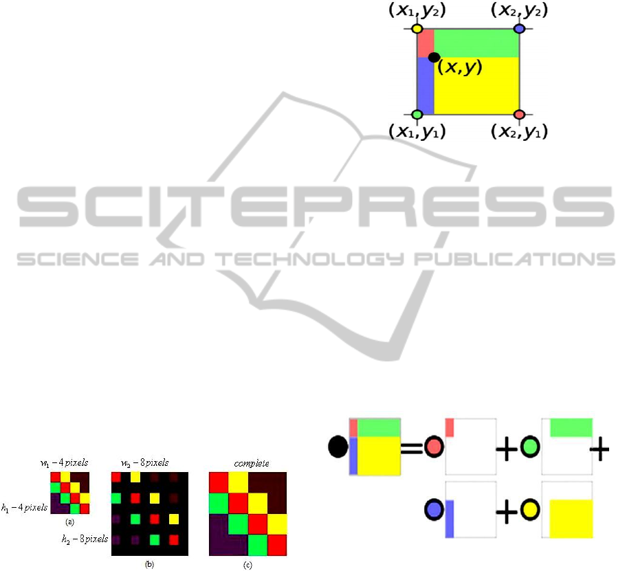
Figure 1: Nearest neighbour interpolation.
Figure 1-(a) with dimension (w1 equals 4, h1
equals 4) has been interpolated at the ratio equal to
two (i.e. w2 equals 8, h2 equals 8). As shown in
Figure 1-(b), the black pixels represent empty spaces
where interpolation is needed, and the complete
Figure 1-(c) is the result of nearest neighbour
interpolation. As one can see, each pixel in the
interpolated image looks doubled when compared to
those belonging to the reference image. This process
requires the shortest time when compared to other
fast interpolation algorithms. Now referring to an
example given in (Bilinear interpolation -Wikipedia,
2012), the unknown pixel value is calculated from
an average of the four neighbours, as shown in
Figure 2.
Figure 2: Unknown pixel location (black dot).
Here,
(
x,
y
)
is the coordinates of the high
resolution pixe
l
whereas ( x
1
, y
2
) ,
(
x
2
, y
2
) , ( x
1
,
y
1
) and ( x
2
, y
1
) are
t
h
e
coordinates of the four
neighbouring low resolution pixe
l
s (yellow,
purple, green and pink dots) surrounding
t
h
e
location of the yet to be high resolution pixel. The
value of the high resolution pixel is calculated
following the process shown in Figure 3. Here, the
value at the black spot (i.e. high resolution pixe
l
) is
the sum of the value at each coloured spot
multiplied by the area of the rectangle of the same
colour, divided by
t
h
e
total area of all four
r
ecta
ngl
e
s.
Figure 3: Calculation of the value of the high resolution
pixel using conventional bilinear interpolation.
Choosing a unit square, the total area of four
rectangles will be equal to one. This simplifies the
traditional bilinear interpolation formula to Eq.1
shown below.
)1,2()2,1()1,1()2,2(
)2,2()1,1()2,1()1,2(),(
yxyxyxyx
yxyxyxyxyx
PWPW
PWPWP
(1)
where,
)1,2( yx
W
,
)1,1( yx
W
,
)2,2( yx
W
and
)2,1( yx
W
represent
the area or weight for the yellow dot
)2,1( yx
P
, purple
VISAPP2014-InternationalConferenceonComputerVisionTheoryandApplications
642
dot
)2,2( yx
P
, green dot
)1,1( yx
P
and pink dot
)1,2( yx
P
. From Eq.1, if:
)()2,1()2,1()2,1()2,1( Nyxyxyxyx
PPPPP
(with
N representing a set of four coordinates
corresponding to the low resolution pixels having
the same value) then Eq.1 can be written as follows.
)(
)2,1()2,2(
)1,1()1,2(
),( N
yxyx
yxyx
yx
P
WW
WW
P
(2)
Since the total area of four rectangles, as shown in
Figure 2 and Figure 3, is equal to one, then Eq.2 can
be simplified as shown by Eq.3.
)(),( Nyx
PP
(3)
where
)( N
P
represent that the gray value common to
all four low resolution pixels, surrounding the empty
location. The simplicity of Eq.3 demonstrates that
the execution time is increased unnecessarily while
using Eq.1 to interpolate all or these four pixels
around the empty location(s). Since, it is believed
this is the source of increased execution time, in this
paper; the authors introduced a decision step so that
those having the same gray values around the empty
location, are not interpolated according to Eq.1 but
Eq.3 (i.e. pixel replication).
3 THE PROPOSED ALGORITHM
The proposed algorithm is developed into three
steps. First, an
nm
source image is divided into
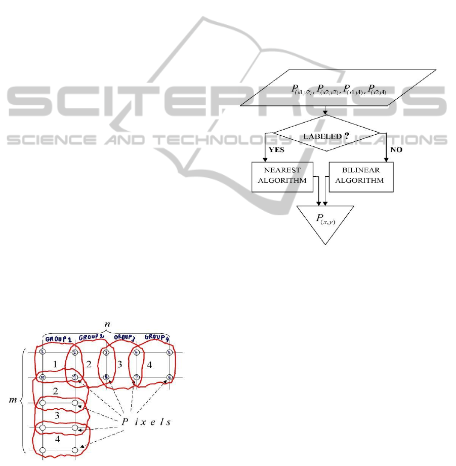
groups of four pixels, as shown in Figure 4.
Figure 4: Pixels grouping.
The number of pixels’ groups comprising that
image is found by first considering the Figure 4;
group 1, group 2, group 3 and group 4, horizontally
a
nd vertically. Here, the difference between the
number of pixels belonging to the first row and the
number of groups touching it is one, and the same
applies for the f
i
rs
t
column. This means that, there
are
m1
groups
t
ouch
i
ng m rows and
n 1
groups
touching
n columns. R
e
f
e
rr
i
ng
to the number of
pixels comprising an
nm
image,
t
h
e
number of
groups is given by the equation b
el
ow.
(1)(1)m n pixels m n groups
(4)
Eq.4 gives the total number of groups to sort. For
each group, if all pixels comprising that group have
the same value, then the nearest neighbour algorithm
is used.
Figure 5: Summary of the proposed algorithm. Here,
‘labeled’ means that; in each group, of four pixels, all the
pixels have the same value.
Else, the bilinear algorithm is used. In other words,
the groups, each having equal values, are labeled to
be processed by nearest neighbour algorithm while
the groups, each having at least one value different
from the others, or unlabeled groups, are processed
by bilinear interpolation. This can be summarized as
shown in below Figure 5 and in this way - with
reference to bilinear algorithm, its performance is
optimized, particularly the speed (see Table 1).
4 EXPERIMENTAL RESULTS
In the experiments, the Peak Signal to Noise Ratio
(PSNR) and Matlab-line Execution Time (MET) are
image quality and speed measures, respectively.
However that image quality and correct interpolation
are two independent aspects. For example, one may
OptimizationofImageInterpolationbasedonNearestNeighbourAlgorithm
643

obtain very nice visual quality even if the
interpolation is imprecise. To verify the precision of
the scheme developed, authors considered the image
interpolation as one preserving the given samples.
This means that if the interpolated signal over the
position of the given samples is subsampled and
subtracted from the subsampled signal, then a
constant signal equivalent to zero must be obtained.
In this case, with the proposed scheme, the
maximum absolute difference equalled to zero (i.e. it
interpolated the given samples, precisely).
Figure 6 shows source/test images used in these
experiments.
The above images, in Figure 6, show an
approximation of the real
images. This is one of
the issues in exploiting digital
images since from
the beginning one does not have or
i
gin
al
reference
whereas the results that look original are des
i
r
e
d.
This issue propagates errors. Thus, the processed
images lose some qualities. The quality of image
can also be lost due to being compressed or
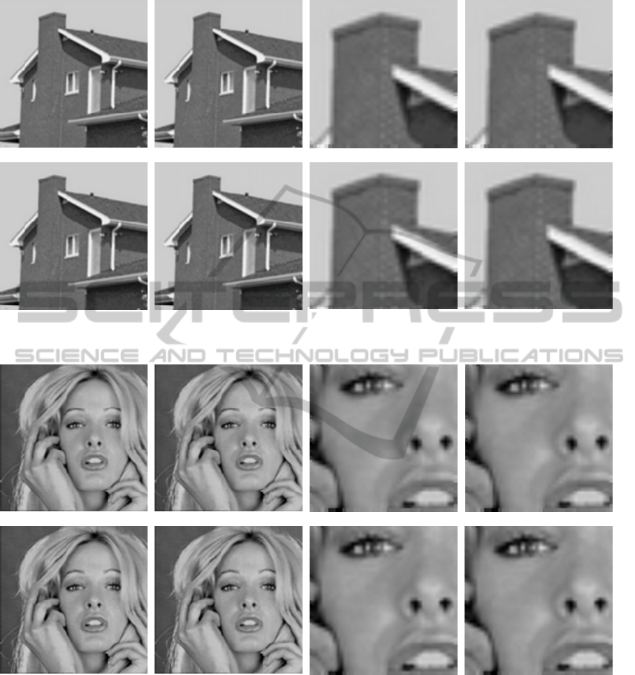
expanded to fit in the desired format. From Figure
7,
i
m
a
ges interpolated by Optimized Bilinear (OB)
algorithm looks sharper than the
i
m
a
ges
interpolated by Conventional Bilinear (CB)
algorithm but still this can be deb
ata
b
le
as to which
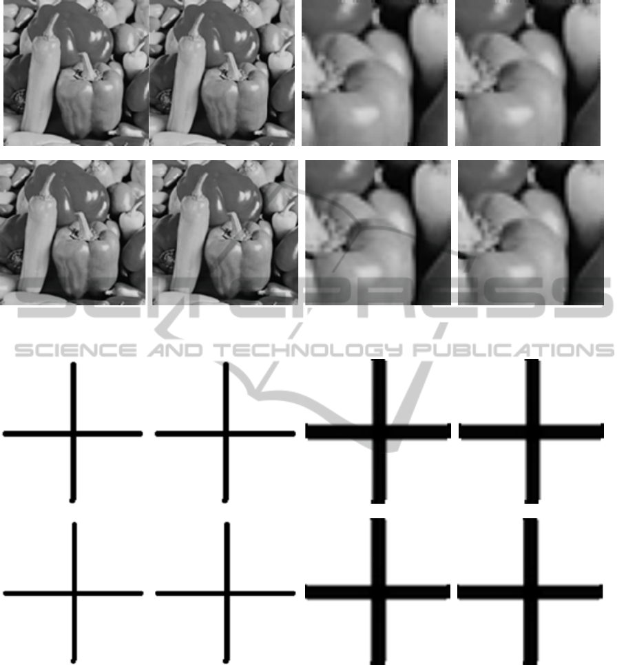
one looks the best. Same for the images shown in
Figure 8 and Figure 9, except the images shown
i
n
Figure 10. In Figure 10, both full and local Cross
i
m
a
ges are interpolated using both mentioned
algorithms at v
a
r
i
ous interpolation ratios. Here,
both algorithms produce
t
h
e
same visual errors.
However, Table 1 and Table 2 prov
e
d that the
PSNR values obtained are not the same. For
e
xampl
e
, when the interpolation ratio equals 4
and Cross image size equals 128 x 128, the OB
algorithm exceeds the CB algorithm by 0.03 dB.
Whereas, for the same interpolation ratio but
at
different image size, that is 40 x 40, it exceeds the
CB by 1.6 dB. In general, this implies that an
algorithm
ca
n perform better for one image size
than another. This kind of situation can be
repeated for the other images (of the s
a
m
e
size or
no
t
).
A part from visual quality, another factor to
determine a good interpolation algorithm is the
processing speed. Theoretically, if the number of
labeled groups is superior to zero, it implies that the
OB speed will be greater than that of the CB.
Furthermore, if the number of the unlabeled groups
is equal to zero, this automatically means that the
OB speeds will be (almost) equal to that of the
nearest neighbour interpolation. However, in
practice, when the number of the unlabeled groups is
equal to zero, it can be seen, from Table 3, that MET
is only about 1.2 times when compared to the CB
algorithm’s MET.
MET values vary depending on the size of image
and interpolation ratio used. For example, with
image size 40 x 40, the number of unlabeled groups
is not equal to zero but one. In this case, MET
is about 1.7 times for interpolation ratio equals
2 and 1.2 when interpolation ratio equals 4.
Table 1: PSNR difference in dB.
Image
names
OB-CB
Full images
Local images
X4 X2 X4 X2
House 0.0784 0.0766 0.1017 0.0796
Girl 0.0125 0.0032 0.0097 0.0223
Peppers 0.0384 0.0162 0.1101 0.0847
Cross 0.0380 0.0004 1.6591 2.0288
Figure 6: Full (128*128) and local (40*40) source images.
VISAPP2014-InternationalConferenceonComputerVisionTheoryandApplications
644
(OB) x4 (CB) x4 (OB) x4 (CB) x4
(OB) x2 (CB) x2 (OB) x2 (CB) x2
Figure 7: Full and local images interpolated by OB and CB.
(OB) x4 (CB) x4 (OB) x4 (CB) x4
(OB) x2 (CB) x2 (OB) x2 (CB) x2
Figure 8: Full and local images interpolated by OB and CB.
5 CONCLUSIONS
An optimization scheme, for (bilinear) image
algorithm, has been proposed in this paper. The
proposed algorithm or scheme includes a decision
step in which it is decided whether the four
neighbouring pixels have the same value and if so,
the conventional bilinear interpolation is replaced
by a nearest neighbour interpolation. Experimental
results demonstrated that the proposed algorithm is
about 1.2 times faster than the CB algorithm which
means that using the CB concept to interpolate all
image pixels indistinctly increases the execution or
processing time. Furthermore, the PSNR values
provided by the OB algorithm are slightly higher
than in the case of the CB algorithm. The reason for
OptimizationofImageInterpolationbasedonNearestNeighbourAlgorithm
645
(OB) x4 (CB) x4 (OB) x4 (CB) x4
(OB) x2 (CB) x2 (OB) x2 (CB) x2
Figure 9: Full and local images interpolated by OB and CB.
(OB) x4 (CB) x4 (OB) x4 (CB) x4
(OB) x2 (CB) x2 (OB) x2 (CB) x2
Figure 10: Full and local images interpolated by OB and CB.
this is that the more one manipulates the image
pixels the more the resulting image quality will be
reduced. This makes the OB algorithm more
appropriate than CB algorithm. And, more
appropriate to relieve the burden of the
computational complexity of other interpolation
schemes, particularly adaptive schemes. During the
experiments there was no need for comparing with
other image interpolation algorithms since the main
concerns was to introduce a scheme that
unsophisticatedly optimizes the CB algorithm
performances, as an example of application based on
this approach. The experimental weakness of the OB
performance however remains the image feature and
size dependence. Future developments of the
proposed scheme can be devoted to optimization
purposes.
VISAPP2014-InternationalConferenceonComputerVisionTheoryandApplications
646

Table 2: This presents the PSNR and MET for different sizes and ratios. The MET value, presented herein, is an average
value. Note, however, that this value can greatly vary depending on external factors such as the processor of a computer
machine used to run the software used, some errors embedded in the version of the software used, etc.
S/F
image
PSNR MET
S/L
image
PSNR MET
x4 x2 x4 x2 x4 x2 x4 x2
CB OB CB OB CB OB CB OB CB OB CB OB CB OB CB OB
House
128 x
128
34.4
103
34.
488
7
34.
726
5
34.
803
1
0.0
854
05
0.0
674
90
0.0
159
12
0.0
148
41
House
40 x 40
33.
360
5
33.
462
2
33.
792
2
33.8
718
0.0
071
89
0.0
065
80
0.0
015
56
0.0
014
82
Girl
128 x
128
32.2
774
32.
289
9
33.
072
9
33.
076
1
0.0
757
09
0.0
707
88
0.0
159
60
0.0
155
65
Girl
40 x 40
33.
485
4
33.
495
1
34.
377
3
34.3
996
0.0
071
75
0.0
067
48
0.0
015
95
0.0
014
27
Peppers
128 x
128
32.6
516
32.
690
0
33.
688
9
33.
705
1
0.0
780
88
0.0
703
92
0.0
158
43
0.0
154
55
Pepper
s
40 x 40
32.
152
7
32.
262
8
33.
124
4
33.2
091
0.0
070
71
0.0
067
91
0.0
015
00
0.0
014
77
Cross
128 x
128
41.3
462
41.
384
2
42.
227
9
42.
228
3
0.0
728
45
0.0
590
96
0.0
155
09
0.0
125
27
Cross
40 x 40
37.
096
6
38.
755
7
39.
216
7
41.2
455
0.0
071
29
0.0
057
99
0.0
023
29
0.0
012
95
Table 3: Speed ratio.
Image
names
OB-CB
Full images Local images
X4 X2 X4 X2
House 1.2654 1.0721 1.0925 1.0499
Girl 1.0695 1.0253 1.0632 1.1177
Peppers 1.1093 1.0251 1.0412 1.0155
Cross 1.2326 1.2380 1.2293 1.7984
REFERENCES
Rukundo, O., Cao, H.Q., 2012. Nearest Neighbor Value
Interpolation. International Journal of Advanced
Computer Science and Applications, Vol. 3, No.4,
pages 25–30.
Lancaster, D., 2012. A Review of Some Image Pixel
Interpolation Algorithms. Available: http://
www.tinaja.com.
Rukundo, O., Wu, K. N., Cao, H. Q., 2011. Image
Interpolation Based On The Pixel Value
Corresponding To The Smallest Absolute Difference.
Presented at the 2011 Fourth International Workshop
on Advanced Computational Intelligence, Wuhan,
China, pages 432-435.
Piedad, B., Iluminada, B., Santiago, S.S., 2007. A Fuzzy
Edge-Dependent Interpolation Algorithm. Studies in
Fuzziness and Soft Computing, 210, pages 157-185.
Sun, G. L., Shen, Z. B., 2010. Single Image Super-
Resolution via Edge Reconstruction and Image
Fusion. Communications in Computer and
Information Science, 123, pages 16-23.
Tschumperle, D., 2002. PDE's Based Regularization of
Multivalued Images and Applications. PhD thesis,
Universite de Nice-Sophia Antipolis, Nice, France.
Morse, B. S., Schwartzwald, D., 1998. Isophote-based
interpolation. In Proc. IEEE International Conference
on Image Processing, Vol. 3, pages 227–231.
Luong, H., De Smet, P., Philips, W., 2005. Image
Interpolation using Constrained Adaptive Contrast
Enhancement Techniques. In Proc. IEEE International
Conference on Image Processing ICIP '05, Genova,
Italy, pages 998-1001.
Alessandro, L., Hiep, Q. L., et al., 2006. Greyscale Image
Interpolation Using Mathematical Morphology.
Springer Lecture Notes in Computer Science, Vol.
4179, pages 78–90.
Shi, Z. F., Yao, S. Y., et al, 2008. A Novel Image
Interpolation Technique Based on Fractal Theory”, In
Proc. IEEE International Conference on Computer
Science and Information Technology, Singapore,
pages 472-475.
Honda, H., Haseyama, M., Kitajima, H., 1999. Fractal
Interpolation for Natural Images”, In Proc. IEEE
International Conference on Image Processing ICIP
'99.Vol. 3, Kobe, Japan, 1999, pp. 657-661.
Noriaki, S., Morihiko, S., Eiji, U., 2008. Image Super-
resolution Based on Local Self-similarity. Optical
Review, Vol. 15, No. 1, pages 26-30.
Stepin, M., 2003. hq3x Magnification Filter. Available
at: http://www.hiend3d.com/hq3x.html.
Freeman, W., Jones, T., Pasztor, E., 2002. Example-Based
Super-Resolution. IEEE Computer Graphics and
Applications, Vol. 22, pages 56-65.
Gabriele, F., Pablo, A., et al., 2009. Exemplar-Based
Interpolation of Sparsely Sampled Images. Springer
Lecture Notes in Computer Science, Vol. 5681, pages
331-344.
Xin, L., Michael T. O., 2001. New Edge-Directed
Interpolation. IEEE Transactions on Image Processing,
Vol. 10, No. 10, pages 1521-1527.
Nearest Neighbor Image Scaling, 2012. Available: <
http://tech-algorithm.com/articles/nearest-neighbor-
image scaling/>
Bilinear interpolation, 2012. Available: <http://
en.wikipedia.org/wiki/Bilinear_interpolation>
OptimizationofImageInterpolationbasedonNearestNeighbourAlgorithm
647
