
Gait Analysis with IMU
Gaining New Orientation Information of the Lower Leg
Steffen Hacker, Christoph Kalkbrenner, Maria-Elena Algorri and Ronald Blechschmidt-Trapp
Institute of Medical Engineering, University of Applied Science Ulm, Albert-Einstein-Allee 55, 89075 Ulm, Germany
Keywords:
Gait Analysis, Inertial Measurement Unit, IMU, Lower Leg.
Abstract:
In this paper we present an application for the analysis and characterisation of gait motion. Using motion data
from Inertial Measurement Units (IMUs), seven relevant parameters are measured that extensively charaterize
the gait of individuals. Our application uses raw and processed IMU data, where the processed data is the
result of filtering the IMU data with a Magdwick filter. The filtered data offers orientation information and is
relatively drift free. The IMU data is used to train a three layer neural network that can then extract individual
footsteps from an IMU dataset. Results with different test persons show that our application can successfully
characterize gait motion on an individual basis and can serve for the clinical assesment and evaluation of
abnormal or pathological gait.
1 INTRODUCTION
Even though human gait is quite similar throughout
each individual, there are still unique parameters in
every single step. These parameters can be investi-
gated to identify an abnormal gait which gives infor-
mation about the health of the patient. Nowadays gait
analysis is often done with optical systems. These
systems can deliver highly accurate data, but camera
systems can only ”see” patients within a limited field
of view. Thus, the use of Inertial Measurement Units
(IMU) is advantageous. These sensors are low-cost
devices and can be worn all day long, without dis-
turbing the patient’s motion. A considerable amount
of literature has been published on gait analysis us-
ing IMUs. IMUs have been used to provide data
for pedestrian tracking, to reconstruct walking routes,
and to analyse the gait of patients with Parkinson’s
disease between many other applications. However,
most of these applications are affected because IMU
measurements tend to drift over time. In 2011 Madg-
wick et al. presented an efficient orientation filter for
IMUs (Madgwick et al., 2011). The benefit of this
filter is that it can extract the orientation information
from the IMU measurements relatively independent
of the presence of drifting. In this work, an appli-
cation is introduced to demonstrate the advantages of
the Madgwick filter in terms of gait analysis. An IMU
based sensor system was mounted on the lower leg
in order to measure its orientation. With this data
new gait parameters such as step height, step distance,
movement path, hip position and velocity could be
obtained.
1.1 Related Work
To date various methods have been developed to mea-
sure gait parameters. Gait analysis with IMUs is
mainly done by analysing raw accelerometer data
(Chung et al., 2012; Sant’Anna et al., 2011; Terada
et al., 2011; Gafurov et al., 2007), which provides
limited information about the gait. Additionally, this
approach requires an accurate orientation of the IMU
in x-, y- and z-axis. Otherwise accelerometer data has
been used as root mean square, which means a com-
plete loss of orientation information.
Fischer et al. describe a method for calculating
the route of a passenger using IMUs (Fischer et al.,
2012). This method requires the usage of a Kalman
Filer to deal with the presence of drift.
Other medical applications of IMU-based gait
analysis have been the measurement of move-
ment symmetry in patients with Parkinson disease
(Sant’Anna et al., 2011) or Alzheimer’s disease
(Chung et al., 2012). There has also been a lot of
interest in the area of general movement analysis with
IMUs, such as upper body motion tracking (Jung
et al., 2010), joint angle measurement (El-Gohary and
McNames, 2012) or fall detection for elderly (Wu and
Xue, 2008).
127
Hacker S., Kalkbrenner C., Algorri M. and Blechschmidt-Trapp R..
Gait Analysis with IMU - Gaining New Orientation Information of the Lower Leg.
DOI: 10.5220/0004787701270133
In Proceedings of the International Conference on Biomedical Electronics and Devices (BIODEVICES-2014), pages 127-133
ISBN: 978-989-758-013-0
Copyright
c
2014 SCITEPRESS (Science and Technology Publications, Lda.)

2 METHOD
In this section we present a new approach for gait
analysis that uses orientation information provided by
data from Inertial Measurement Units (IMUs). The
data from the IMUs is first processed using a Madg-
wick Filter (Madgwick et al., 2011) to produce only
the orientation (3D rotation) information of the IMU.
The IMU orientation information is fed into a neu-
ronal network to find and characterize individual foot-
steps in long sets of data obtained from the IMUs. Af-
ter individual steps are identified in the data sequence,
each step is analysed in terms of step length, velocity,
lateral amplitude and movement path.
2.1 Position of the IMU
To best identify footsteps in motion tracking data pro-
vided by IMUs, there are two possible positions to
place the IMU: Foot and lower leg. The position at
the lower leg (see fig. 6) offers more robust motion
tracking data, since orientation measurements at the
foot itself can be distorted as the foot adapts itself to
rough terrain while walking. This circumstance can
induce errors in the recognition of footsteps, as the
foot undergoes slight rotations that are not related to
the gait itself when walking over uneven ground. In
addition to this, from placement of the IMU on the
lower leg we will be able to reconstruct the position
and orientation of the lower extremity. For these rea-
sons, our method uses data from IMUs mounted on
the lower leg (as shown in figure 6), although this is
contrary to the common position of IMUs at the foot,
such as found in (Chung et al., 2012; Patterson and
Caulfield, 2011).
2.2 Step Recognition
After the IMU data is processed with the Madgwick
Filter, we are left with a rotation matrix M
R
that gives
the 3D orientation of the sensor itself. From the ma-
trix M
R
the direction of the sensor coordinate system,
with axes x
s
,y
s
and z
s
can easily be determined at any
given time. This coordinate system is defined by the
rotation of the axes in the global coordinate system
(fig. 1), which is determined by the Madgwick Filter,
once the sensor unit connects. Accordingly, the angle
ω between the lower leg and the direction of gravity
can also be calculated, as can be seen in fig. 6. There-
fore, the vector corresponding to the direction of the
lower leg
~
l can be initially assigned on the basis of the
sensor axes information while the subject stands still.
Assuming that the lower leg is perpendicular to the
surface or respectively, parallel to the gravity acceler-
y
s
x
s
z
s
y
z
x
sensor unit
Figure 1: Global coordinate system and sensor coordinate
system.
ation while the subject is standing upright, the vector
of the lower leg can be determined as the scalar prod-
uct,
l
x
=
~x
s
·~z
|
~x
s
|
|~z|
, l
y
=
~y
s
·~z
|
~y
s
|
|~z|
, l
z
=
~z
s
·~z
|
~z
s
|
|~z|
, (1)
with z = (0,0,−1), the vector of gravity acceleration.
The angle ω between
~
l and~z is used for step recogni-
tion.
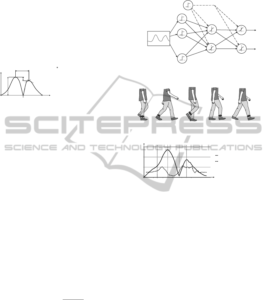
Although there are several pattern recognition
techniques that can be used to identify footsteps,
we are limited by the fact that footsteps must be
characterized individually from subject to subject.
For this reason, a three layer feed forward neural
network was designed in order to characterize and
find steps of different persons in motion tracking
datasets. Another possible solution would use sup-
ported vector machines, as seen in (Begg et al., 2005)
and (Wu, 2012). The recognition of a distinct pattern
in a dataset can be seen as a classification problem
(Bishop, 2006). In this case there are two possible
classes that a dataset can be classified into: contains
a footstep and does not contain a footstep. Since a
dataset is obtained by recording a subject’s gait over
several minutes, there are many footsteps to be found
in the post processing. In order to find each step,
the dataset is divided into sequences of 200 samples
each, which represent two seconds of motion with a
sampling frequency of 100 Hz. If no step is found
inside a sequence k in the database (where k is the
position of the first sequence sample in the dataset),
a new sequence is taken starting at sample k + 10, as
can be seen in figure 2.
data
sequence
classifcation
neural
network
no step: k+10; step: k+200
k
Figure 2: Step recognition using a sequence of 200 data
points inside a long dataset.
In the case that a footstep is identified in the 200
sample sequence k, the next sequence to be input
to the neural network starts at sample k + 200. Se-
BIODEVICES2014-InternationalConferenceonBiomedicalElectronicsandDevices
128
quences are input into the neural network, until the
end of the dataset is reached. Features are extracted
from each sequence in order to fasten the learning
process of the neural network. To extract features
from a sequence, we find all the extrema of ω(t)
and calculate specific parameters such as distance be-
tween maxima or the gradient of certain sections. An
overview of the feature extraction can be seen in fig.
3. If the feature being learned is a continuous one,
t
angle
extrema
1
2
3
4
1 proportion of maxima
2 value of maximum
3 distance of maxima
4 gradient of curve before
4
and after extrema
Figure 3: Overview of the most important features that are
extracted from a sequence.
like a gradient or a distance, the firing neurons are
dependent on the continuous input value. For exam-
ple, when the feature that we want to characterize (we
want the neural network to learn) is a gradient m
x
of a
section before a minimal turning point, the firing neu-
rons could be defined as:
N[n] = 1 if: m
x
< 1
N[n+1] = 1 if: 1 < m
x
< 2
N[n+2] = 1 if: 2 < m
x
< 3
.
.
.
N[n+9] = 1 if: m
x
> 10
As can be seen, continuous features of the curve,
such as proportion of maximal turning points or gradi-
ent before minimal turning points, are assigned to an
amount of 8-10 input neurons, although the number of
input neurons adapt to the variability of the continu-
ous signal. Finally all features together lead up to 110
input neurons. The hidden layer of the neural network
improves the recognition of patterns if classes need to
be separated multidimensionally. The hidden layer in
this application consists of 10 neurons, with the sig-
modial activation function:
f
act
(net) =
1
1 + e
−net
(2)
With the addition of a threshold of 1, the resulting
neural network can be seen in fig. 4. The learning rate
of the neural network is the factor that influences the
convergence of the learned features. It is set to 0.1,
as advised in (Bishop, 2006). Using the described
feature extraction process, only a small number of
input data was required to train the network. After
50 patterns of various footsteps were presented to the
network, footsteps in an arbitrary dataset were found
sequence
hidden layer
input neurons
n = 110
n = 10
n = 2
threshold
output layer
.
.
.
step
no step
n = 200 datapoints
.
.
.
Figure 4: Neural network with three layers.
0
20
40
60
40 80 120
1
2
3
4
5
frames
angle ω in
◦
acceleration in m/s
2
1
2
3
4
5
Figure 5: Angle of the lower leg to z-axis and root means
square of acceleration data during a step.
with an exactness of 94%. Each learning sequence
that was used to train the network was trimmed, so
that it represented a motion sequence as seen in fig. 5.
2.3 Step Parameter Calculation
It is possible to extract various features of a step using
the orientation information from the IMUs. In the fol-
lowing, the x- and y-axes are located in the transversal
plane (corresponding to the floor plane) and the z-axis
is defined in the direction of gravity, perpendicular to
~x and~y. x, y and z-axes are defined as the global coor-
dination system, and x
s
, y
s
and z
s
-axes are the sensor
axes, see fig. 1.
2.3.1 Direction
The direction of a step, which we define as the pro-
visional movement direction vector
~
d
∗
, can be deter-
mined by projecting the vector of the lower leg
~
l to
the x/y-plane (fig. 7) The angle θ inside the x/y-plane
can be determined as:
GaitAnalysiswithIMU-GainingNewOrientationInformationoftheLowerLeg
129

h
s,v
h
s
ω
h
f
a
Figure 6: Parameters of foot height computation at a spe-
cific time.
x
y
~
d
∗
θ
x
θ
y
Figure 7: Top view of the vectors for receiving movement
direction. The orientation of the global coordinate system x
and y-axes is defined by the Madgwick Filter as explained
above.
θ
x
= arccos
~x ·
~
d
∗
|
~x
|
|
~
d
∗
|
and θ
y
= arccos
~y ·
~
d
∗
|
~y
|
|
~
d
∗
|
(3)
Since there are four quadrants in the x/y plane, a dis-
tinction of cases needs to be done in order to find the
correct angle of movement direction θ:
θ =
θ = θ
x
if θ
x
< 90
◦
and θ
y
< 90
◦
θ = θ
x
if θ
x
> 90
◦
and θ
y
< 90
◦
θ = θ
y
+ 90
◦
if θ
x
> 90
◦
and θ
y
> 90
◦
θ = 360
◦
− θ
x
if θ
x
< 90
◦
and θ
y
> 90
◦
(4)
With θ already known, the vector of movement direc-
tion
~
d can be calculated as,
~
d =
cosθ
sinθ
0
(5)
2.3.2 Step Length
The vertical position of the sensor s
r
(t) at a given time
t during a step is the double integration of the accel-
eration a
d
(t), in the direction of movement. Accord-
ingly the final step length s
r
is the position of the foot
at the end of the step. The acceleration data in x
s
,
y
s
and z
s
-direction is directly obtained from the IMU.
The acceleration in the direction of movement a
d
can
simply be maintained by calculating the dot product
of the x
s
and y
s
axes with
~
d. Afterwards these two
ratios are each multiplied with the measured acceler-
ation a
x
respectively a
y
. Therefore, the step length
s
r
(t) is:
s
r
(t) =
Z
t
0
Z
t
0
a
d
(t)dt dt
(6)
2.3.3 Route
The route can simply be maintained by multiplying
the direction vector
~
d with the final step length s
r
. The
route is built as a sequence of points representing the
history of the motion direction in the x/y plane. A new
route point P
n+1
(x,y) in x and y-direction is calculated
as:
P
n+1
(x) = P
n
(x) +
~
d
x
s
r
P
n+1
(y) = P
n
(y) +
~
d
y
s
r
(7)
2.3.4 Step Height
The vertical position of the sensor h
s
(t) during a step
can be obtained by double integration of the accelera-
tion a
z
(t) in the z direction:
h
s
(t) =
Z
t
0
Z
t
0
a
z
(t)dt dt (8)
Since the sensor is placed on the lower leg and not on
the foot itself, the vertical position of the foot h
f
(t)
cannot be measured directly. First, the vertical posi-
tion of the sensor needs to be calculated. With l
L
the
known length of the lower leg, and ω(t
∗
) the angle be-
tween lower leg and the z-axis, the distance a of the
sensor to the knee (center of lower leg rotation) is:
a =
s
h
s
(t
∗
)
cos
−
1
2
ω(t
∗
)
2
1
2(1 − cos(−
1
2
ω(t
∗
)))
(9)
In this case, a is calculated at a specific time (t
∗
),
where the angle ω(t) is maximal. Therefore the height
of the sensor h
s,v
from the sole of the foot can be ob-
tained with:
h
s,v
= l
L
− a; (10)
Now the height of the foot h
f
(t) over time can be ob-
tained with:
h
f
(t) = (h
s,v
+ h
s
(t)) − cos(ω)h
s,v
(11)
This means that the position of the sensor (a couple
of centimeters higher or lower) can vary and we will
still be able to get a correct measurement of h
f
(t). An
overview of the calculated parameters can be seen in
fig. 6.
BIODEVICES2014-InternationalConferenceonBiomedicalElectronicsandDevices
130

2.3.5 Foot Position in Movement Direction
Analogous to the height h
f
of the foot, the position
s
f
of the foot can be calculated. In order to get s
f
a
distinction of cases with respect to the angle ω must
be taken into account. ω is defined negative if the foot
position is posterior and positive if the foot position is
anterior.
s
f
(t)
(
s
r
(t) − sin(|ω|)h
s,v
for ω < 0
s
r
(t) + sin(|ω|)h
s,v
for ω > 0
(12)
2.3.6 Lateral Amplitude
The lateral amplitude s
l
(t) can be defined as the an-
gle of the foot to the plane parallel to the direction
of movement. That means, the dot product between
the direction of movement ~r and the gravitation vec-
tor~z needs to be calculated, in order to obtain the nor-
mal vector ~n
d
of the plane parallel to the direction of
movement.
~n
d
=~r ×~z (13)
Afterwards the angle between the lower leg vector
~
l
and ~n
d
can be easily computed as seen in (3). This
angle is the lateral amplitude, which indicates if a pa-
tient has limping gait or not.
2.3.7 Position of Thigh
With the vertical foot position s
f
(t), the horizontal
foot position h
f
(t) and the angle ω(t) at any given
time, the gait can be visualized. But since there is
only one sensor placed on the lower leg, the position
of the thigh needs to be predicted. Using the results of
gait analysis (Perry, 2003) a best-fit curve of the angle
γ(p) between the lower leg vector vec(l) and the thigh
is determined. The angle γ(p) is determined with re-
spect to the step phase p (expressed as a percentage).
γ(p) =
175
◦
for p < 20%
f (p) for 20% < p < 75%
175
◦
for p > 75%
(14)
with f (p) a polynomial of the 5th order:
f (p) = 4.1 · 10
−6
p
5
− 9.8 · 10
−3
p
4
+
0.1p
3
− 3.4p
2
+ 56.3p − 153.4 (15)
Thereby the position of the thigh (and hip) can be rea-
sonably approximated. Some of the calculated param-
eters can be seen in fig. 8. As can be seen, the angle
ω(t) and the lateral amplitude over time give addi-
tional information about the gait.
~
d
plain of movement
direction
~n
d
in lateral
direction
posterior
anterior
Figure 8: Gait parameters. The lateral amplitude is defined
as the angle between the lower leg and z-axis in direction of
~n
d
.
3 RESULTS
The proposed methodology allows a near complete
characterization of the different gait parameters. For
instance one single step of a 25 year old male subject
results in the following parameters:
step length: 1.38 m
max. posterior amplitude (fig. 5 (3)): 43
◦
max. anterior amplitude (fig. 5 (5)) 40
◦
max step height h
s
: 24 cm
step duration: 1.17 s
average velocity: 1.18 m/s
The corresponding graph of one single step can be
seen in fig. 9.
Figure 9: Step analysis. The developed application com-
putes step length, step duration, max. lateral amplitude and
average velocity. Furthermore a graphical output gives in-
formation about the angle ω(t), acceleration (rms) and lat-
eral amplitude over time.
To validate the algorithms three subjects were re-
quested to walk ten steps along a straight line. The
sensor was placed on the left lower leg. Afterwards
the distance was measured and the results were com-
pared using the computed step length of a whole step
GaitAnalysiswithIMU-GainingNewOrientationInformationoftheLowerLeg
131

Table 1.
subject distance calculated difference
1 13.70 m 14.10 m 2.9%
2 13.30 m 13.96 m 4.9%
3 12.90 m 13.38 m 3.7%
Figure 10: Movement paths, top view. left: walking over a
straight line with different step length. right: walking an s-
shape trajectory. The black line marks the beginning. Each
step ends with a dot, so that different step lengths can be
seen.
s
r
. As can be seen in Table 1, there is an average error
of 3.8% percent between the actual walked distance
and the calculated distance. That is about 4 cm of
error measurement at every step.
Additionally sensor orientation is used to detect
the direction of movement. One subject was re-
quested to walk in a straight line with small steps
at the beginning, normal step size in the middle and
small steps at the end. As can be seen in fig. 10
the route and the variability in step length can easily
be determined. The developed algorithm works with
non-linear walking routes as well, as can be seen to
the right of fig. 10. For this figure, the subject was
asked to walk an s-shape trajectory with normal step
size. The walking route was determined using the al-
gorithm presented here.
4 CONCLUSIONS
Using raw IMU information and IMU information fil-
tered with a Madgwick filter we were able to outline
a new application to extensively characterize gait pa-
rameters that provide new information about leg ori-
entation and movement direction.
In the future we suggest more studies to outline
the limitations of the developed application. The al-
gorithm for gait analysis needs to be tested with vari-
ous pathological patients and with the results of such
tests, there will be a possibility to automatise long-
term gait analysis. With that in mind, patients suffer-
ing from conditions whose severity can be at least par-
tially assessed by continuous gait analysis can profit
from the monitoring application presented in this pa-
per.
ACKNOWLEDGEMENTS
The authors would like to thank Karl Dubies and
Michael Stuber for assistance with the data acquisi-
tion. This work was supported by a grant from the
Ministry of Science, Research and the Arts of Baden-
Wuerttemberg (Az: 33-7533-7-11.6-10/2).
REFERENCES
Begg, R., Palaniswami, M., and Owen, B. (2005). Sup-
port vector machines for automated gait classifica-
tion. Biomedical Engineering, IEEE Transactions on,
52(5):828–838.
Bishop, C. M. (2006). Pattern recognition and machine
learning. Springer, New York, NY.
Chung, P.-C., Hsu, Y.-L., Wang, C.-Y., Lin, C.-W., Wang,
J.-S., and Pai, M.-C. (2012). Gait analysis for patients
with alzheimer’s disease using a triaxial accelerome-
ter. In Circuits and Systems (ISCAS), 2012 IEEE In-
ternational Symposium on, pages 1323–1326.
El-Gohary, M. and McNames, J. (2012). Shoulder
and elbow joint angle tracking with inertial sen-
sors. Biomedical Engineering, IEEE Transactions on,
59(9):2635–2641.
Fischer, C., Talkad Sukumar, P., and Hazas, M. (2012). Tu-
torial: implementation of a pedestrian tracker using
foot-mounted inertial sensors. Pervasive Computing,
IEEE, PP(99):1–1.
Gafurov, D., Snekkenes, E., and Bours, P. (2007). Spoof
attacks on gait authentication system. Informa-
tion Forensics and Security, IEEE Transactions on,
2(3):491–502.
Jung, Y., Kang, D., and Kim, J. (2010). Upper body mo-
tion tracking with inertial sensors. In Robotics and
Biomimetics (ROBIO), 2010 IEEE International Con-
ference on, pages 1746–1751.
Madgwick, S., Harrison, A. J. L., and Vaidyanathan, R.
(2011). Estimation of imu and marg orientation us-
ing a gradient descent algorithm. In Rehabilitation
Robotics (ICORR), 2011 IEEE International Confer-
ence on, pages 1–7.
Patterson, M. and Caulfield, B. (2011). A novel approach
for assessing gait using foot mounted accelerometers.
In Pervasive Computing Technologies for Healthcare
(PervasiveHealth), 2011 5th International Conference
on, pages 218–221.
Perry, J. (2003). Ganganalyse: Norm und Pathologie des
Gehens. Urban & Fischer, Munich, 1. aufl. edition.
Sant’Anna, A., Salarian, A., and Wickstrom, N. (2011). A
new measure of movement symmetry in early parkin-
son’s disease patients using symbolic processing of
inertial sensor data. Biomedical Engineering, IEEE
Transactions on, 58(7):2127–2135.
Terada, S., Enomoto, Y., Hanawa, D., and Oguchi, K.
(2011). Performance of gait authentication using an
acceleration sensor. In Telecommunications and Sig-
nal Processing (TSP), 2011 34th International Con-
ference on, pages 34–36.
BIODEVICES2014-InternationalConferenceonBiomedicalElectronicsandDevices
132

Wu, G. and Xue, S. (2008). Portable preimpact fall detector
with inertial sensors. Neural Systems and Rehabilita-
tion Engineering, IEEE Transactions on, 16(2):178–
183.
Wu, J. (2012). Automated recognition of human gait pattern
using manifold learning algorithm. In Natural Com-
putation (ICNC), 2012 Eighth International Confer-
ence on, pages 199–202.
GaitAnalysiswithIMU-GainingNewOrientationInformationoftheLowerLeg
133
