
Empirical Study of Domain Adaptation with Na
¨
ıve Bayes on the Task of
Splice Site Prediction
Nic Herndon and Doina Caragea
Kansas State University, Computing and Information Sciences, 234 Nichols Hall, Manhattan, KS 66506, U.S.A.
Keywords:
Domain Adaptation, Na
¨
ıve Bayes, Splice Site Prediction, Unbalanced Data.
Abstract:
For many machine learning problems, training an accurate classifier in a supervised setting requires a sub-
stantial volume of labeled data. While large volumes of labeled data are currently available for some of these
problems, little or no labeled data exists for others. Manually labeling data can be costly and time consuming.
An alternative is to learn classifiers in a domain adaptation setting in which existing labeled data can be lever-
aged from a related problem, referred to as source domain, in conjunction with a small amount of labeled data
and large amount of unlabeled data for the problem of interest, or target domain. In this paper, we propose two
similar domain adaptation classifiers based on a na
¨
ıve Bayes algorithm. We evaluate these classifiers on the
difficult task of splice site prediction, essential for gene prediction. Results show that the algorithms correctly
classified instances, with highest average area under precision-recall curve (auPRC) values between 18.46%
and 78.01%.
1 INTRODUCTION
In recent years, a rapid increase in the volume of dig-
ital data generated has been observed. Gantz et al.
(2007) estimated that the total volume of digital data
doubles every 18 months. Contributing to this growth,
in the field of biology, large amounts of raw genomic
data are generated with next generation sequencing
technologies, as well as data derived from primary se-
quences. The availability and scale of the biological
data creates great opportunities in terms of medical,
agricultural, and environmental discoveries, to name
just a few.
A stepping stone towards advancements in such
fields is the identification of genes in a genome. Ac-
curate identification of genes in eukaryotic genomes
depends heavily on the ability to accurately determine
the location of the splice sites (Bernal et al., 2007;
R
¨
atsch et al., 2007), the sections in the DNA that sep-
arate exons from introns in a gene. In addition to iden-
tifying the gene structure, the splice sites also deter-
mine the amino acid composition of the proteins en-
coded by the genes. Therefore, considering that the
content of a protein plays a major role with respect
to its function, the splice site prediction is a crucial
task in identifying genes and ultimately the functions
of their products.
To identify genes, we need to identify two types
of splice sites: donor and acceptor. The donor splice
site indicates where an exon ends and an intron be-
gins, while the acceptor splice site indicates where an
intron ends, and an exon begins. Virtually most donor
sites are the GT dimer and most acceptor sites are the
AG dimer, with very few exceptions. However, not
every GT or AG dimer is a splice site. In fact, only
about one percent of them are, which makes the task
of identifying splice sites very difficult.
Nonetheless, this problem can be addressed with
supervised machine learning algorithms, which have
been successfully used before for many biological
problems, including gene prediction. For example,
hidden Markov models have been used for ab ini-
tio gene predictions, while support vector machines
(SVMs) have been used successfully for problems
such as identification of translation initiation sites
(M
¨
uller et al., 2001; Zien et al., 2000), labeling
gene expression profiles as malign or benign (Noble,
2006), ab initio gene prediction (Bernal et al., 2007),
and protein function prediction (Brown et al., 2000).
However, one drawback of these algorithms is that
they require large amounts of labeled data to learn
accurate classifiers. And many times labeled data is
not available for a problem of interest, yet it is avail-
able for a different but related problem. For example,
in biology, a newly sequenced organism is generally
scarce in labeled data, while a well-studied model or-
57
Herndon N. and Caragea D..
Empirical Study of Domain Adaptation with Naïve Bayes on the Task of Splice Site Prediction.
DOI: 10.5220/0004806800570067
In Proceedings of the International Conference on Bioinformatics Models, Methods and Algorithms (BIOINFORMATICS-2014), pages 57-67
ISBN: 978-989-758-012-3
Copyright
c
2014 SCITEPRESS (Science and Technology Publications, Lda.)

ganism is rich in labeled data. However, the use of
the classifier learned for the related problem to clas-
sify unlabeled data for the problem of interest does
not always produce accurate predictions. A better al-
ternative is to learn a classifier in a domain adaptation
(DA) framework. In this setting, the large corpus of
labeled data from the related, well studied organism
is used in conjunction with available labeled and un-
labeled data from the new organism.
Towards this goal we propose two similar algo-
rithms, described in Section 3.2. Each algorithm
trains a classifier in this configuration, by using the
large volume of labeled data from a well studied or-
ganism, also called source domain, some labeled data,
and any available unlabeled data from the new organ-
ism, called target domain. Once learned, the classifier
can be used to classify new data from the new organ-
ism. These algorithms are similar to the algorithms
in (Tan et al., 2009; Herndon and Caragea, 2013a;
Herndon and Caragea, 2013b), which produced good
results on the tasks of sentiment analysis and protein
localization, respectively.
For example, the algorithm proposed by Hern-
don and Caragea (2013b) uses a weighted multino-
mial Na
¨
ıve Bayes classifier combined with the itera-
tive approach of the Expectation-Maximization algo-
rithm and self-training (Yarowsky, 1995; Riloff et al.,
2003; Maeireizo et al., 2004). It iterates until the
probabilities in the expectation step converge. In the
maximization step, the posterior probabilities and the
likelihood are estimated using a weighted combina-
tion between the labeled data from the source domain
and the labeled and unlabeled data from the target do-
main. In the expectation step, the conditional class
probabilities for each instance in the target unlabeled
dataset are estimated with the probability values from
the maximization step using Bayes theorem. After
each iteration, a number of instances from the unla-
beled target dataset are considered labeled and moved
to the labeled dataset. The number of these instances
is proportional to the prior probability, with a mini-
mum of one instance selected from each class. For
example, if the target labeled dataset had 1% positive
instances and 99% negative instances, and at each it-
eration we select 10 instances, one instance with the
top positive probability and nine instances with the
top negative probabilities would be selected. In addi-
tion, the weight is shifted from the source data to the
target data with each iteration.
However, this algorithm did not perform well on
the task of splice site prediction and to improve its
classification accuracy we made the following four
changes to it:
• We normalized the counts used in computing the
posterior probability and the likelihood, and as-
signed different weights to the target labeled and
unlabeled datasets.
• We used mutual information to rank the features
instead of the marginal probabilities of the fea-
tures.
• We assigned different weights to the features in-
stead of selecting which features to use from the
source domain.
• We used features that took into consideration the
location of nucleotides instead of counts of 8-mers
generated with a sliding window.
With these changes, the two algorithms produced
promising results, shown in Section 3.5, when eval-
uated on the splice site prediction problem with the
data presented in Section 3.3. They increased the
highest average auPRC from about 1% in (Herndon
and Caragea, 2013b) all the way up to 78.01%.
2 RELATED WORK
Although there are good domain adaptation results
for text classification, even with algorithms that make
significant simplifying assumptions, such as na
¨
ıve
Bayes, there are only a few domain adaptation algo-
rithms designed for biological problems. For exam-
ple, for text classification, Dai et al. (2007) proposed
an algorithm that combined na
¨
ıve Bayes (NB) with
expectation-maximization (EM) for classifying text
documents into top categories. This algorithm per-
formed better than SVM and na
¨
ıve Bayes classifiers.
Two other domain adaptation algorithms that used a
combination of NB with EM are (Tan et al., 2009),
which produced promising results on the task of sen-
timent analysis of text documents, and (Herndon and
Caragea, 2013a), with good results on the task of pro-
tein localization.
However, for the task of splice site prediction, up
until now, most of the work used supervised learning
classifiers with only two exceptions in domain adap-
tation setting to the best of our knowledge: one that
analyzed several support vector machine algorithms
(Schweikert et al., 2008), and another that used na
¨
ıve
Bayes (Herndon and Caragea, 2013b). The latter did
not obtain good results, primarily due to the features
generated. It used the number of occurrences in each
instance of the k-mers of length eight generated with
a sliding window.
For supervised learning, Li et al. (2012) evaluated
the discriminating power of each position in the DNA
sequence around the splice site using the chi-square
test. With this information, they proposed a SVM
BIOINFORMATICS2014-InternationalConferenceonBioinformaticsModels,MethodsandAlgorithms
58

algorithm with a RBF kernel function that used a
combination of scaled component features, nucleotide
frequencies at conserved sites, and correlative infor-
mation of two sites, to train a classifier for the hu-
man genome. Other supervised learning approaches
based on SVM include (Baten et al., 2006; Sonnen-
burg et al., 2007; Zhang et al., 2006), while (Cai et al.,
2000) proposed an algorithm for splice site prediction
based on Bayesian networks, (Baten et al., 2007) pro-
posed a hidden Markov model algorithm, and (Arita
et al., 2002) proposed a method using Bahadur ex-
pansion truncated at the second order. However, su-
pervised learning algorithms typically require a large
volume of labeled data to train a classifier.
For domain adaptation setting, Schweikert et al.
(2008) obtained good results using a SVM with
weighted degree kernel (R
¨
atsch and Sonnenburg,
2004), especially when the source and target domains
were not close. However, the complexity of SVM
classifiers increases with the number of training in-
stances and the number of features, when training the
classifier (Schweikert et al., 2008). Besides, the clas-
sification results are not as easy to interpret as the re-
sults of probabilistic classifiers, such as na
¨
ıve Bayes,
to gain insight into the problem studied. For example,
Scheikert et al. (2008) further processed the results to
analyze the relevant biological features. In addition,
their algorithms did not use the large volume of tar-
get unlabeled data. Although unlabeled, this dataset
could improve the classification accuracy of the algo-
rithm.
3 METHODOLOGY
The two algorithms we propose are based on the al-
gorithm presented in our previous work (Herndon and
Caragea, 2013b). That algorithm modified the al-
gorithm introduced by (Tan et al., 2009), by using
self-training and the labeled data from the target do-
main, to make it suitable for biological sequences. To
highlight the changes made to our previous algorithm
we’ll describe it here.
3.1 Na
¨
ıve Bayes DA for Biological
Sequences
The algorithm in (Herndon and Caragea, 2013b) was
designed to use labeled data from the source domain
in conjunction with labeled and unlabeled data from
the target domain to build a classifier to be used on the
target domain. It is an iterative algorithm that uses a
combination of the Bayes’ theorem with the simplify-
ing assumption that features are independent, and the
expectation-maximization algorithm (Dempster et al.,
1977), to estimate the posterior probability as propor-
tional to the product of the prior and the likelihood:
P(c
k
| d
i
) ∝ P(c
k
)
|V |
∏
t=1
[P(w
t
| c
k
)]
N
T
t,i
(1)
where the prior is defined as
P(c
k
) =
(1 − λ)
|D
S
|
∑
i
0
=1
P(c
k
| d
i
0
) + λ
|D
T
|
∑
i
00
=1
P(c
k
| d
i
00
)
(1 − λ)|D
S
| + λ|D
T
|
(2)
and the likelihood is defined as
P(w
t
| c
k
) =
(1 − λ)(η
t
N
S
t,k
) + λN
T
t,k
+ 1
(1 − λ)
|V |
∑
t=1
η
t
N
S
t,k
+ λ
|V |
∑
t=1
N
T
t,k
+ 1
(3)
where λ is a weight factor between the two domains:
λ = min{δ · τ, 1}
τ is the iteration number, with a value of 0 for the
first iteration, and δ ∈ (0, 1) is a constant that indicates
how fast the weight of the source domain decreases
while the weight of the target domain increases; c
k
stands for class k, d
i
for document i, and w
t
for feature
t.
|D
x
| is the number of instances in x domain (x ∈
{S, T }, where S denotes the source domain and T de-
notes the target domain), |V | is the number of features,
and N
x
t,k
is the number of times feature w
t
occurs in x
domain in instances labeled with class c
k
:
N
x
t,k
=
|D
x
|
∑
i=1
N
x
t,i
P(c
k
| d
i
)
N
x
t,i
is the number of occurrences in x domain of fea-
ture w
t
in instance d
i
.
η
t
=
(
1, if feature w
t
is generalizable.
0, otherwise.
To determine which features from the source do-
main are generalizable to the target domain, i.e., gen-
eralizable from use on D
S
to use on D
T
, they are
ranked with the following measure and only the top
ranking features are kept:
f (w
t
) = log
P
S
(w
t
) · P
T
(w
t
)
|P
S
(w
t
) − P
T
(w
t
)| + α
(4)
where α is a small constant used to prevent division
by 0 when P
S
= P
T
, and P
x
is the probability of fea-
ture w
t
in x domain, i.e., the number of times feature
w
t
occurs in x domain divided by the sum over all fea-
tures of the times each feature occurs in x domain.
EmpiricalStudyofDomainAdaptationwithNaïveBayesontheTaskofSpliceSitePrediction
59

This algorithm iterates until convergence. In the
maximization step, the prior and likelihood are si-
multaneously estimated using Equations 2 and 3, re-
spectively, while in the expectation step the posterior
for the target unlabeled instances is estimated using
Equation 1. In addition to expectation-maximization,
this algorithm uses self-training, i.e., at each itera-
tion it selects a number of unlabeled instances with
highest class probabilities, proportional to the class
distribution, and considers them to be labeled during
subsequent iterations, while the remaining unlabeled
instances are assigned “soft labels” for the following
iteration. By soft labels we mean that the class prob-
ability distribution is used instead of the class label.
For the target domain, during the first iteration, only
the instances from the labeled dataset are used, and
for the rest of the iterations, instances from both la-
beled and unlabeled datasets are used.
Note that when the algorithm goes through just
one iteration and λ = 1, the prior and likelihood Equa-
tions, 2 and 3, respectively, reduce to
P(c
k
) =
|D
S
|
∑
i=1
P(c
k
| d
i
)
|D
S
|
(5)
and
P(w
t
| c
k
) =
|D
S
|
∑
i=1
N
t,i
P(c
k
| d
i
) + 1
|V |
∑
t=1
|D
S
|
∑
i=1
N
t,i
P(c
k
|d
i
) + |V |
(6)
respectively, which are the equations for the multi-
nomial na
¨
ıve Bayes classifier (Mccallum and Nigam,
1998) trained and tested with data from the same do-
main.
Although the algorithm in (Herndon and Caragea,
2013b) performed well on the task of protein localiza-
tion with maximum auPRC values between 73.98%
and 96.14%, on the task of splice site prediction, the
algorithm performed poorly. The splice site predic-
tion is a more difficult task because only about 1%
of the AG dimer occurrences in a genome are splice
sites. To simulate this proportion, unbalanced datasets
were used, with each containing only about 1% pos-
itive instances. Therefore, the training sets for splice
site prediction were much more unbalanced than the
training sets for the protein localization, leading to
worse performance for the former.
3.2 Our Approach
One major drawback of the algorithm in (Herndon
and Caragea, 2013b) is that it assigns low weight to
the target data (through λ in Equations 2 and 3), in-
cluding the labeled data, during the first iterations.
This biases the classifier towards the source domain.
However, it is not effective to only assign a differ-
ent weight to the target labeled data in Equations 2
and 3. This is because we’d like to use much more
instances from the source domain as well as much
more unlabeled instances from the target domain, i.e.,
|D
S
| |D
T L
| and |D
TU
| |D
T L
|, where subscripts S,
T L, and TU stand for source data, target labeled data,
and target unlabeled data, respectively. This would
cause the sums and counts for the target labeled data
in these two equations to be much smaller than their
counterparts for the source data and target unlabeled
data, rendering the weight assignment useless. In-
stead, we need to also normalize these values, or bet-
ter yet, to use their probabilities. Thus, we estimate
the prior as
P(c
k
) = βP
T L
(c
k
)+(1−β)[(1−λ)P
S
(c
k
)+λP
TU
(c
k
)]
(7)
and the likelihood as
P(w
t
| c
k
) = βP
T L
(w
t
| c
k
)
+ (1 − β)[(1 − λ)P
S
(w
t
| c
k
) + λP
TU
(w
t
| c
k
)]
(8)
where β ∈ (0, 1) is a constant weight, and λ is defined
the same as in our previous approach.
In addition to using different formulas for prior
and likelihood, we made a second change to the algo-
rithm in (Herndon and Caragea, 2013b). We replaced
the measure for ranking the features, Equation 4, with
the following measure in Equation 9. We made this
change because the goal of ranking the features is to
select top features in terms of their correlation with
the class, or assign them different weights: higher
weights to features that are more correlated with the
class, and lower weights to the features that are less
correlated with the class. Therefore, the mutual in-
formation (Shannon, 1948) of each feature is a more
appropriate measure in determining the correlation of
the feature with the class rather than the marginal
probability of the feature. With this new formula, the
features are ranked better based on their generalizabil-
ity between the source and target domains:
f (w
t
) =
I
S
(w
t
;c
k
) · I
T L
(w
t
;c
k
)
|I
S
(w
t
;c
k
) − I
T L
(w
t
;c
k
)| + α
(9)
where
I
x
(w
t
, c
k
) =
|V |
∑
t=1
|C|
∑
k=1
P
x
(w
t
, c
k
)log
P
x
(w
t
, c
k
)
P
x
(w
t
)P
x
(c
k
)
is the mutual information between feature w
t
and
class c
k
, and x ∈ {S, T L}. The numerator ranks higher
BIOINFORMATICS2014-InternationalConferenceonBioinformaticsModels,MethodsandAlgorithms
60

the features that have higher mutual information in
their domains, while the denominator ranks higher the
features that have closer mutual information between
the domains, as shown in Figure 1.
If instead of ranking the features and using the top
ranked features, we want to assign different weights
to the features and higher values for f (w
t
) we can
compute them with the formula in Equation 10. For
the splice site prediction problem using the data from
Section 3.3 with the features described in Section 3.4,
most of the mutual information values are close to
zero since each feature contributes very little to the
classification of an instance. Therefore, the nomi-
nator is about one order of magnitude smaller than
the denominator in Equation 9, while in Equation 10,
the numerator is close to the denominator, resulting in
higher values for f (w
t
).
The final change we made to (Herndon and
Caragea, 2013b) was the use of different features, as
explained shortly in Section 3.4.
f (w
t
) =
I
S
(w
t
;c
k
) · I
T L
(w
t
;c
k
)
(I
S
(w
t
;c
k
) − I
T L
(w
t
;c
k
))
2
+ α
(10)
Thus, the two algorithms we propose use the
source labeled data and the target labeled and unla-
beled data to train a classifier for the target domain.
For the source domain, Algorithm 1 selects general-
izable features to be used, while Algorithm 2 assigns
different weights to the features. These differences
are highlighted in italics in steps 1 and 2 of the al-
gorithms by using italics text. The algorithms iter-
ate until convergence. In the first iteration, they use
only the source and target labeled data to calculate
and assign the posterior probabilities for the unlabeled
data. Proportional to the prior probability distribution,
the algorithms select top instances from the target un-
labeled dataset and consider them to be labeled for
subsequent iterations. For the rest of the iterations,
the algorithms use the source labeled data, the target
labeled data, and the target unlabeled data to build
a classifier for labeling the remaining unlabeled in-
stances. For the target unlabeled data, the algorithms
use the probability distributions, while for the other
datasets, source and target labeled, they use the labels
of each instance when computing the prior probabili-
ties and the likelihood.
3.3 Data Set
To evaluate these algorithms, we used a dataset for
which (Herndon and Caragea, 2013b) did not perform
well. We used the splice site dataset
1
, first introduced
1
Downloaded from ftp://ftp.tuebingen.mpg.de/fml/
cwidmer/
Algorithm 1: DA with feature selection.
1: Select the features to be used from the source domain
using Equation 9.
2: Simultaneously compute the prior and likelihood,
Equations 7 and 8, respectively. Note that for the
source domain all labeled instances are used but only
with the features selected in step 1, while for the tar-
get domain only labeled instances are used with all
their features.
3: Assign labels to the unlabeled instances from the tar-
get domain using Equation 1. Note that we use self-
training, i.e., a number of instances, proportional to
the class distribution, with the highest class proba-
bility are considered to be labeled in subsequent it-
erations.
4: while labels assigned to unlabeled data change do
5: M-step: Same as step 2, except that we also use
the instances in the target unlabeled dataset; for
this dataset we use the class for the self-trained
instances, and the class distribution for the rest of
the instances.
6: E-step: Same as step 3.
7: end while
8: Use classifier on new target instances.
Algorithm 2: DA with weighted features.
1: Assign different weights to the features of the
source dataset using either Equation 9 or Equa-
tion 10.
2: Simultaneously compute the prior and likelihood,
Equations 7 and 8, respectively. Note that for the
source domain all labeled instances are used but
the features are assigned different weights in step
1, while for the target domain only labeled in-
stances are used with all their features.
3: Assign labels to the unlabeled instances from the
target domain using Equation 1. Note that we use
self-training, i.e., a number of instances, propor-
tional to the class distribution, with the highest
class probability are considered to be labeled in
subsequent iterations.
4: while labels assigned to unlabeled data change
do
5: M-step: Same as step 2, except that we
also use the instances in the target unlabeled
dataset; for this dataset we use the class for the
self-trained instances, and the class distribution
for the rest of the instances.
6: E-step: Same as step 3.
7: end while
8: Use classifier on new target instances.
in (Schweikert et al., 2008), which contains DNA se-
quences of 141 nucleotides long, with the AG dimer
EmpiricalStudyofDomainAdaptationwithNaïveBayesontheTaskofSpliceSitePrediction
61
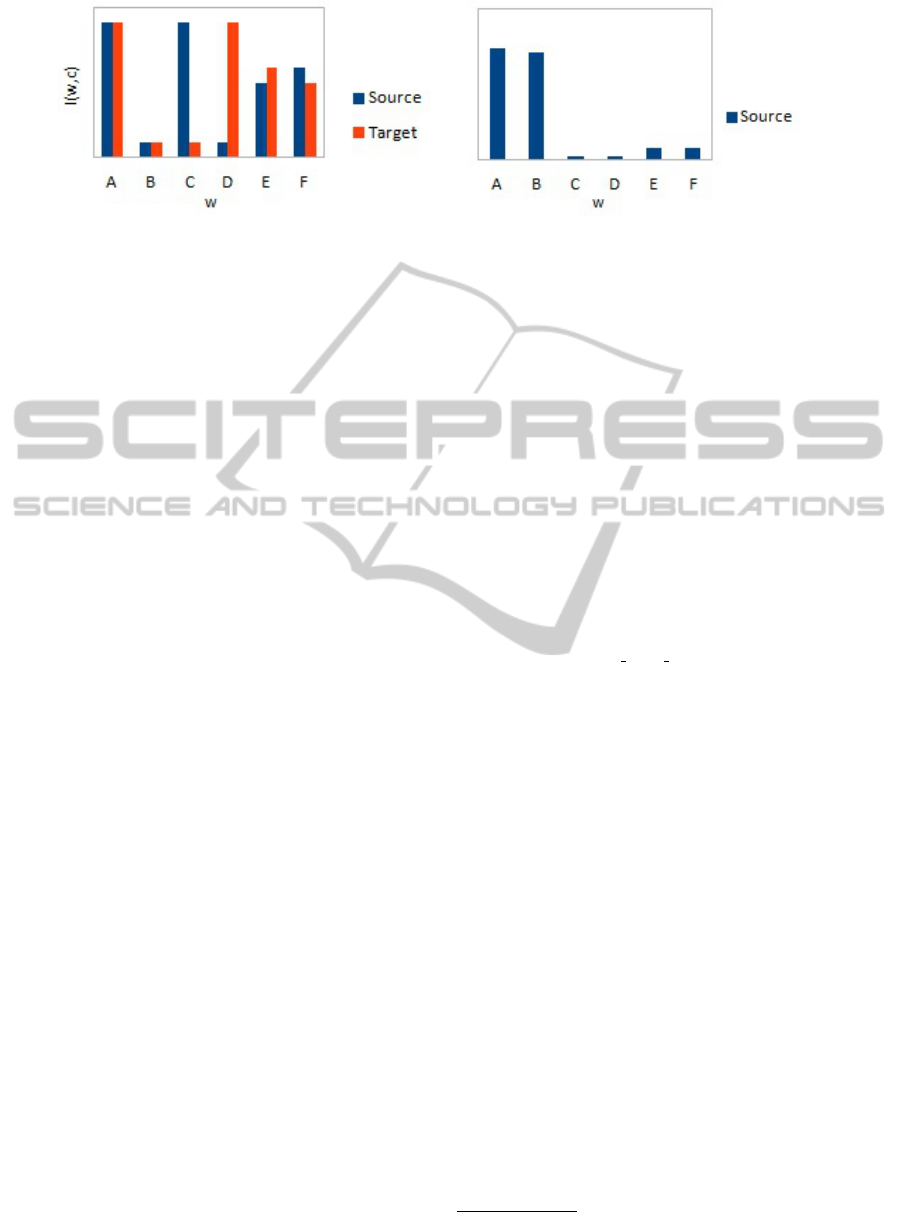
(a) Mutual information of features in both domains (b) Rank of features in the source domain
Figure 1: Ranking features in the source domain based on mutual information using Equation 9, showcasing the different
combinations of mutual information of the features in the two domains. Feature A has high mutual information in both
domains, as shown on the left of subfigure (a), resulting in large numerator and small denominator, and thus a high rank, as
shown on the left of subfigure (b). Feature B has low mutual information in both domains, resulting in small denominator,
and thus a high rank, but lower than the rank of A since the numerator for A is greater than the numerator for B. Features
C and D have high mutual information in one domain and low mutual information in the other domain, resulting in large
denominator, and thus a low rank. Features E and F have close mutual information between the two domains, resulting in
small denominator, and thus a higher rank than Features C and D.
at sixty-first position in the sequence, and a class label
that indicates whether this dimer is an acceptor splice
site or not. Although this dataset contains only accep-
tor splice sites, classifying donor splice sites can be
done similarly to classifying the acceptor splice sites.
This dataset contains sequences from one source
organism, C.elegans, and four target organisms at in-
creasing evolutionary distance, namely, C.remanei,
P.pacificus, D.melanogaster, and A.thaliana. The
source organism contains a set of 100,000 instances,
while each target organism has three folds each of
1,000, 2,500, 6,500, 16,000, 25,000, 40,000, and
100,000 instances that can be used for training, as
well as three corresponding folds of 20,000 instances
to be used for testing. In each file, there are 1% posi-
tive instances with small variations – variance is 0.01
– and the remaining instances are negative.
3.4 Data Preparation and Experimental
Setup
To limit the number of experiments, we used the fol-
lowing datasets, as shown in Figure 2:
• The 100,000 C.elegans instances as source la-
beled data used for training.
• Only the sets with 2,500, 6,500, 16,000, and
40,000 instances as labeled target data used for
training.
• The set with 100,000 instances as unlabeled target
data used for training.
• The corresponding folds of the 20,000 instances
as target data used for testing.
We represent each sequence as a combination
of features that indicate the nucleotide and codon
present at each location, i.e., 1-mer and 3-mer,
respectively. We chose these features to create a
balanced combination of simple features, 1-mers,
and features that capture some correlation between
the nucleotides, 3-mers, while keeping the number of
features small. For example, a sequence starting with
AAGATTCGC... and class –1 would be represented
in WEKA ARFF
2
format as:
@RELATION remanei
2500 0
@ATTRIBUTE NUCLEOTIDE1 {A,C,G,T}
.
.
.
@ATTRIBUTE NUCLEOTIDE141 {A,C,G,T}
@ATTRIBUTE CODON1 {AAA,AAC,. . .,TTT}
.
.
.
@ATTRIBUTE CODON138 {AAA,AAC,. . .,TTT}
@ATTRIBUTE cls {1,-1}
@DATA
A,A,G,A,T,T,C,G,C,. . .,AAG,AGA,GAT,. . .,-1
In our previous work we used a bag-of-words ap-
proach with k-mers of length eight. This led to 4
8
or
65,535 sparse features. Moreover, those features did
not take into consideration the location of each nu-
cleotide. We believe that the major improvement we
achieved is due to the features used, fewer and more
location-aware.
We ran two different experiments
with a grid search for the optimal val-
ues for β ∈ {0.1, 0.2, . . . , 0.9} and δ ∈
{0.01, 0.02, . . . , 0.08, 0.09, 0.1, 0.2}. In the first
one, we used only the nucleotides as features, while
2
WEKA Attribute-Relation File Format (ARFF) is de-
scribed at http://www.cs.waikato.ac.nz/ml/weka/arff.html
BIOINFORMATICS2014-InternationalConferenceonBioinformaticsModels,MethodsandAlgorithms
62
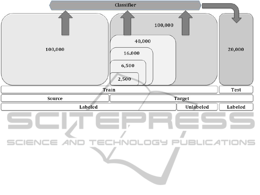
Figure 2: Experimental setup. Our algorithms are trained on the source labeled dataset (100,00 instances) from C.elegans,
target labeled instances (2,500, 6,500, 16,000, or 40,000 instances) and target unlabeled instances (100,000 instances) from
C.remanei, P.pacificus, D.melanogaster, or A.thaliana. Once trained, each algorithm is tested on 20,000 instances from the
corresponding target dataset.
in the second one we used nucleotides and codons
as features. In both settings, we ran Algorithm 1
to select the features in the source domain (A1),
Algorithm 2 using Equation 9 to weigh the features
in the source domain (A2E9), and Algorithm 2 with
Equation 10 to weigh the source domain features
(A2E10).
To ensure that our results are unbiased, we re-
peated the experiments three times with different
training and test splits. We used two baselines to eval-
uate our classifiers. The first baseline, which we ex-
pect to represent the lower bound, is the na
¨
ıve Bayes
classifier trained on the target labeled data (NBT). We
believe that this will be the lower bound for our clas-
sifiers because we expect that adding the labeled data
from a related organism (the source domain) as well
as unlabeled data from the same organism (the tar-
get domain) should produce a better classifier. The
second baseline is the na
¨
ıve Bayes classifier trained
on the source labeled data (NBS). We expect that
the more distantly related the two organisms are, the
less accurate the classifier trained on the source data
would be when tested on the target data.
Our goal with this experimental setup was to de-
termine how each of the following influence the per-
formance of the classifier:
1. Features used, i.e., nucleotides, or nucleotides and
codons.
2. Algorithm used, i.e., Algorithm 1 which keeps
only the generalizable features in the source do-
main, or Algorithm 2 which assigns different
weights to the features in the source domain.
3. Number of target labeled instances used in train-
ing the classifier, i.e., 2,500, 6,500, 16,000, or
40,000.
4. The evolutionary distance between the source and
target domains.
5. Using source labeled data and target unlabeled
data when training the classifier.
3.5 Results
Since the class distribution is highly skewed, with
each set containing about 1% positive instances and
the rest, about 99%, negative instances, we used the
area under the precision-recall curve as a metric for
evaluating the accuracy of our classifiers, and we
present the highest auPRCs averaged over the three
folds.
In Table 1, we list the auPRC for our classi-
fiers, the best overall algorithm in (Schweikert et al.,
2008), SVM
S,T
, and for the classifiers in (Hern-
don and Caragea, 2013b). An additional view, that
presents the trends of our classifiers, is shown in the
Appendix. Although our results are not as good as the
ones in (Schweikert et al., 2008), they are greatly im-
proved compared to results in (Herndon and Caragea,
2013b), yet not as much as we expected. Even though
they are not as good as the SVM
S,T
in (Schweikert
et al., 2008), they could be superior in some con-
texts. In addition, as we mentioned in Section 2,
the complexity of SVM classifiers increases with the
number of training instances and the number of fea-
tures, when training the classifier (Schweikert et al.,
EmpiricalStudyofDomainAdaptationwithNaïveBayesontheTaskofSpliceSitePrediction
63

Table 1: auPRC values for four target organisms based on the number of labeled target instances used for training: 2,500,
6,500, 16,000, and 40,000. The tables on the left (a, c, g, and e) show the values for the algorithms trained with nucleotide
features, while the tables on the right (b, d, f, and h) show the values for the algorithms trained with nucleotide and codons
features. NBT and NBS are baseline na
¨
ıve Bayes classifiers trained on target labeled and source data, respectively, for the two
algorithms we proposed, Algorithm 1 (A1) and Algorithm 2 (A2E9 and A2E10 when using Equation 9 and 10, respectively).
We show for comparison with our algorithms the values for the best overall algorithm in (Schweikert et al., 2008), SVM
S,T
,
and the values in (Herndon and Caragea, 2013b), ANB. Note that these values are shown in each table even though the
SVM
S,T
and ANB algorithms used different features.
2,500 6,500 16,000 40,000
ANB 1.13 1.13 1.13 1.10
NBT 23.42 45.44 54.57 59.68
A1 59.18 63.10 63.95 63.80
A2E9 35.03 46.08 54.89 59.73
A2E10 48.92 60.83 63.06 63.59
NBS 63.77
SVM 77.06 77.80 77.89 79.02
2,500 6,500 16,000 40,000
ANB 1.13 1.13 1.13 1.10
NBT 22.94 58.39 68.40 75.75
A1 45.29 72.00 74.83 77.07
A2E9 24.96 61.45 69.11 75.91
A2E10 49.22 70.23 75.43 78.01
NBS 77.67
SVM 77.06 77.80 77.89 79.02
(a) C.remanei (nucleotides) (b)C.remanei (nucleotides+codons)
2,500 6,500 16,000 40,000
ANB 1.00 0.97 1.07 1.10
NBT 19.22 37.33 45.33 52.84
A1 45.32 49.82 52.09 54.62
A2E9 19.85 37.51 45.64 52.91
A2E10 37.20 48.71 52.31 55.62
NBS 49.12
SVM 64.72 66.39 68.44 71.00
2,500 6,500 16,000 40,000
ANB 1.00 0.97 1.07 1.10
NBT 26.39 48.54 59.29 68.78
A1 20.21 53.29 62.33 69.88
A2E9 20.16 43.95 57.44 65.80
A2E10 20.19 57.21 65.99 70.94
NBS 67.10
SVM 64.72 66.39 68.44 71.00
(c) P.pacificus (nucleotides) (d) P.pacificus (nucleotides+codons)
2,500 6,500 16,000 40,000
ANB 1.07 1.13 1.07 1.03
NBT 14.90 26.05 35.21 39.42
A1 33.31 36.43 40.32 42.37
A2E9 16.27 26.21 35.12 39.16
A2E10 22.86 32.92 36.95 37.55
NBS 31.23
SVM 40.80 37.87 52.33 58.17
2,500 6,500 16,000 40,000
ANB 1.07 1.13 1.07 1.03
NBT 13.87 25.00 35.28 45.85
A1 25.83 32.58 39.10 47.49
A2E9 15.03 26.45 34.73 42.90
A2E10 22.53 29.47 36.18 42.92
NBS 34.09
SVM 40.80 37.87 52.33 58.17
(e) D.melanogaster (nucleotides) (f) D.melanogaster (nucleotides+codons)
2,500 6,500 16,000 40,000
ANB 1.20 1.17 1.20 1.17
NBT 7.20 17.90 28.10 34.82
A1 18.46 25.04 31.47 36.95
A2E9 8.42 18.39 28.22 34.79
A2E10 13.61 22.28 29.05 34.66
NBS 11.97
SVM 24.21 27.30 38.49 49.75
2,500 6,500 16,000 40,000
ANB 1.20 1.17 1.20 1.17
NBT 3.10 8.76 28.11 40.92
A1 3.99 13.96 33.62 43.20
A2E9 2.65 8.72 29.39 40.35
A2E10 3.64 10.00 30.85 40.40
NBS 13.98
SVM 24.21 27.30 38.49 49.75
g) A.thaliana (nucleotides) h) A.thaliana (nucleotides+codons)
2008). While their algorithms “required an equivalent
of about 1,500 days of computing time on state-of-
the-art CPU cores” to tune their parameters (Schweik-
ert et al., 2008), and additional computing to analyze
the biological features, our algorithms required the
equivalent of only 300 days of computing, and the
results can be easily interpreted. Furthermore, we be-
lieve that our algorithms are interesting from a theo-
retical perspective and it is useful to know how well
they perform.
Based on these results, we make the following ob-
servations:
1. Using a classifier with both the nucleotides and
the codons as features performs better as the size
of the target labeled data increases, while a clas-
sifier using only the nucleotides as features per-
forms better with smaller target labeled datasets.
We believe that this is caused by the fact that the
codon features are sparser than the nucleotide fea-
tures, and when there is little target labeled data
the classifier does not have enough data to sepa-
rate the positive from the negative instances.
BIOINFORMATICS2014-InternationalConferenceonBioinformaticsModels,MethodsandAlgorithms
64

2. The A1 classifier, based on Algorithm 1, and
the A2E10 classifier, based on Algorithm 2, per-
formed better than the other classifier, A2E9, each
producing the best results in 11 and 5 cases, re-
spectively. As mentioned above, the sparsity of
the data affects the performance of the classi-
fiers based on the features used. The A1 classi-
fier, which uses only the nucleotides as features,
performs better when the target labeled dataset
is small, and also when the two organisms are
more distantly related, while the A2E10 classifier,
which uses the nucleotides and codons as features,
performs better when the target labeled dataset is
larger and the two organisms are more closely re-
lated.
3. The general trend in all classifiers is that they per-
form better as more target labeled instances are
used for training. This conforms with our intu-
ition that using a small dataset for training does
not produce a good classifier.
4. As the evolutionary distance increases between
the source and target organisms, the performance
of our classifiers decreases. When the source and
target organisms are closely related, as is the case
with C.elegans and C.remanei, the large volume
of labeled source data significantly contributes to
generating a better classifier, compared to train-
ing a classifier on the target data alone. How-
ever, as the source and target organisms diverge,
the source data contributes less to the classifier.
5. Using the source data and the target unlabeled
data in addition to the target labeled data im-
proves the performance of the classifier (e.g., A1
v. NBT for A.thaliana with 2,500 instances) com-
pared to training a classifier on just the target la-
beled data. The improvement occurs even with
larger datasets, although less substantial than with
smaller datasets.
4 CONCLUSIONS AND FUTURE
WORK
In this paper, we presented two similar domain adap-
tation algorithms based on the na
¨
ıve Bayes classifier.
They are based on the algorithms in (Herndon and
Caragea, 2013a; Herndon and Caragea, 2013b), to
which we made four changes. The first change was
to use probabilities for computing the prior and like-
lihood, Equations 7 and 8, instead of the counts in
Equations 2 and 3. The second change was to use
mutual information in Equations 9 and 10 instead of
marginal probabilities to rank the features in Equation
4. The third change was to assign different weights
to the features from the source domain instead of se-
lecting the features to use during training. The final
change was to use fewer but more informative fea-
tures. We used nucleotides and codons features that
are aware of their location in the DNA sequence in-
stead of 8-mers generated with a sliding window ap-
proach.
With these changes, we significantly improved the
classification performance as compared to (Herndon
and Caragea, 2013b). In addition, empirical results
on the splice site prediction task support our hypoth-
esis that augmenting a small labeled dataset with a
large labeled dataset from a close domain and unla-
beled data from the same domain improves the per-
formance of the classifier. This is especially the case
when we have small amounts of labeled data but the
same trend occurs for larger labeled datasets as well.
In future work, we would like to more thoroughly
evaluate the predictive power of the features we used,
and to investigate whether other algorithms might
produce better results when used with these features.
To evaluate the features, we plan to use data from
other organisms, and also shuffle the existing data and
the labels, and see how this affects the performance of
the classifiers. To identify algorithms that might po-
tentially be better for the task addressed in this work,
we will investigate other transfer learning algorithms
and compare their results with the results of our pro-
posed algorithms.
In addition, we would like to further improve our
classifier and are considering three approaches. In one
approach, besides the features derived from biologi-
cal background, nucleotides (1-mers) and codons (3-
mers), we would like to use additional features, such
as 2-mers, for example, or biological features, such
as pyrimidine-rich motifs around the acceptor splice
site. In another approach, we would like to address
the splice site prediction problem as an anomaly de-
tection problem, since the preponderance of positive
instances is so small. And in the final approach, we
would like to balance the ratio of positive and nega-
tive instances going as far as using only the positive
labeled data for training.
ACKNOWLEDGMENTS
The computing for this project was performed on the
Beocat Research Cluster at Kansas State University,
which is funded in part by NSF grants CNS-1006860,
EPS-1006860, EPS-0919443, and MRI-1126709.
EmpiricalStudyofDomainAdaptationwithNaïveBayesontheTaskofSpliceSitePrediction
65

REFERENCES
Arita, M., Tsuda, K., and Asai, K. (2002). Modeling splic-
ing sites with pairwise correlations.
Baten, A., Chang, B., Halgamuge, S., and Li, J. (2006).
Splice site identification using probabilistic parame-
ters and SVM classification.
Baten, A. K., Halgamuge, S. K., Chang, B., and Wickra-
marachchi, N. (2007). Biological Sequence Data Pre-
processing for Classification: A Case Study in Splice
Site Identification. In Proceedings of the 4th inter-
national symposium on Neural Networks: Part II–
Advances in Neural Networks, ISNN ’07, pages 1221–
1230, Berlin, Heidelberg. Springer-Verlag.
Bernal, A., Crammer, K., Hatzigeorgiou, A., and Pereira, F.
(2007). Global Discriminative Learning for Higher-
Accuracy Computational Gene Prediction. PLoS
Comput Biol, 3(3):e54.
Brown, M. P. S., Grundy, W. N., Lin, D., Cristianini, N.,
Sugnet, C., Furey, T. S., M.Ares, J., and Haussler,
D. (2000). Knowledge-based Analysis of Microar-
ray Gene Expression Data Using Support Vector Ma-
chines. PNAS, 97(1):262–267.
Cai, D., Delcher, A., Kao, B., and Kasif, S. (2000). Model-
ing splice sites with Bayes networks. Bioinformatics,
16(2):152–158.
Dai, W., Xue, G., Yang, Q., and Yu, Y. (2007). Transfer-
ring Na
¨
ıve Bayes Classifiers for Text Classification.
In Proceedings of the 22nd AAAI Conference on Arti-
ficial Intelligence.
Dempster, A. P., Laird, N. M., and Rubin, D. B. (1977).
Maximum Likelihood from Incomplete Data via the
EM Algorithm. Journal of the Royal Statistical Soci-
ety. Series B (Methodological), 39(1):1–38.
Gantz, J. H., Reinsel, D., Chute, C., Schlinchting, W.,
McArthur, J., Minton, S., Xheneti, I., Toncheva, A.,
and Manfrediz, A. (2007). The Expanding Digital
Universe.
Herndon, N. and Caragea, D. (2013a). Na
¨
ıve Bayes Domain
Adaptation for Biological Sequences. In Proceedings
of the 4th International Conference on Bioinformatics
Models, Methods and Algorithms, BIOINFORMAT-
ICS 2013, pages 62–70.
Herndon, N. and Caragea, D. (2013b). Predicting pro-
tein localization using a domain adaptation approach.
Communications in Computer and Information Sci-
ence (CCIS 2013). Springer-Verlag.
Li, J., Wang, L., Wang, H., Bai, L., and Yuan, Z. (2012).
High-accuracy splice site prediction based on se-
quence component and position features. Genet Mol
Res, 11(3):3432–51.
Maeireizo, B., Litman, D., and Hwa, R. (2004). Co-training
for predicting emotions with spoken dialogue data. In
Proceedings of the ACL 2004 on Interactive poster
and demonstration sessions, ACLdemo ’04, Strouds-
burg, PA, USA. Association for Computational Lin-
guistics.
Mccallum, A. and Nigam, K. (1998). A Comparison of
Event Models for Na
¨
ıve Bayes Text Classification. In
AAAI-98 Workshop on ’Learning for Text Categoriza-
tion’.
M
¨
uller, K.-R., Mika, S., R
¨
atsch, G., Tsuda, S., and
Sch
¨
olkopf, B. (2001). An Introduction to Kernel-
Based learning Algorithms. IEEE Transactions on
Neural Networks, 12(2):181–202.
Noble, W. S. (2006). What is a support vector machine?
Nat Biotech, 24(12):1565–1567.
R
¨
atsch, G. and Sonnenburg, S. (2004). Accurate Splice
Site Prediction for Caenorhabditis Elegans. In Kernel
Methods in Computational Biology, MIT Press series
on Computational Molecular Biology, pages 277–298.
MIT Press.
R
¨
atsch, G., Sonnenburg, S., Srinivasan, J., Witte, H.,
M
¨
uller, K.-R., Sommer, R., and Sch
¨
olkopf, B. (2007).
Improving the C. elegans genome annotation using
machine learning. PLoS Computational Biology,
3:e20.
Riloff, E., Wiebe, J., and Wilson, T. (2003). Learning sub-
jective nouns using extraction pattern bootstrapping.
In Proceedings of the seventh conference on Natural
language learning at HLT-NAACL 2003 - Volume 4,
CONLL ’03, pages 25–32, Stroudsburg, PA, USA.
Association for Computational Linguistics.
Schweikert, G., Widmer, C., Sch
¨
olkopf, B., and R
¨
atsch, G.
(2008). An Empirical Analysis of Domain Adapta-
tion Algorithms for Genomic Sequence Analysis. In
NIPS’08, pages 1433–1440.
Shannon, C. E. (1948). A mathematical theory of commu-
nication. The Bell System Technical Journal, 27:379–
423, 623–656.
Sonnenburg, S., Schweikert, G., Philips, P., Behr, J., and
R
¨
atsch, G. (2007). Accurate Splice site Prediction Us-
ing Support Vector Machines. BMC Bioinformatics,
8(Supplement 10):1–16.
Tan, S., Cheng, X., Wang, Y., and Xu, H. (2009). Adapt-
ing Na
¨
ıve Bayes to Domain Adaptation for Sentiment
Analysis. In Proceedings of the 31th European Con-
ference on IR Research on Advances in Information
Retrieval, ECIR ’09, pages 337–349, Berlin, Heidel-
berg. Springer-Verlag.
Yarowsky, D. (1995). Unsupervised word sense disam-
biguation rivaling supervised methods. In Proceed-
ings of the 33rd annual meeting on Association for
Computational Linguistics, ACL ’95, pages 189–196,
Stroudsburg, PA, USA. Association for Computa-
tional Linguistics.
Zhang, Y., Chu, C.-H., Chen, Y., Zha, H., and Ji, X. (2006).
Splice site prediction using support vector machines
with a Bayes kernel. Expert Syst. Appl., 30(1):73–81.
Zien, A., R
¨
atsch, G., Mika, S., Sch
¨
olkopf, B., Lengauer, T.,
and M
¨
uller, K.-R. (2000). Engineering support vec-
tor machine kernels that recognize translation initia-
tion sites. Bioinformatics, 16(9):799–807.
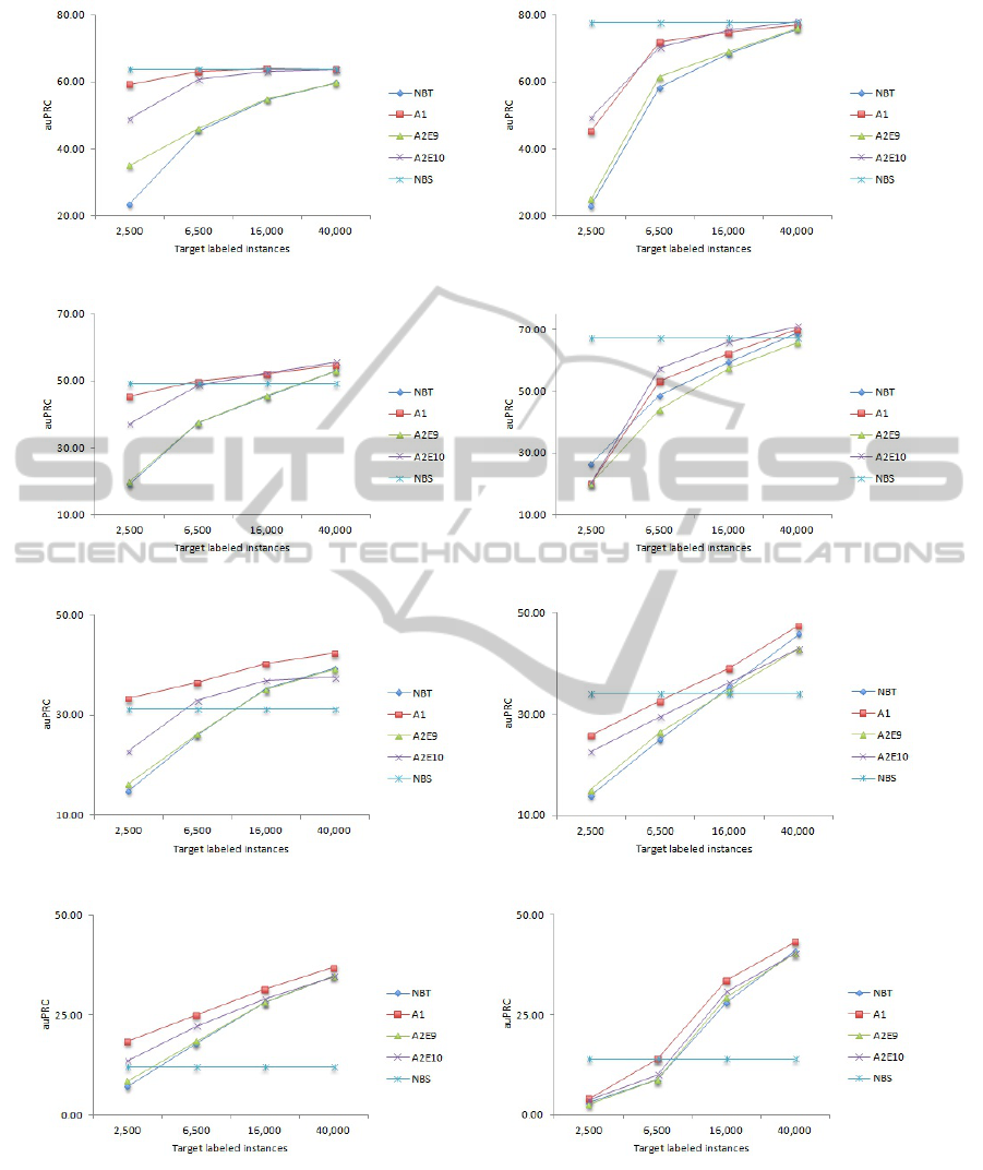
APPENDIX
In this appendix we show the trends in our classifier
based on the size of the target labeled dataset and the
features used.
BIOINFORMATICS2014-InternationalConferenceonBioinformaticsModels,MethodsandAlgorithms
66
(a) C.remanei (nucleotides) (b) C.remanei (nucleotides+codons)
(c) P.pacificus (nucleotides) (d) P.pacificus (nucleotides+codons)
(e) D.melanogaster (nucleotides) (f) D.melanogaster (nucleotides+codons)
(g) A.thaliana (nucleotides) (h) A.thaliana (nucleotides+codons)
Figure 3: auPRC for four target organisms when using nucleotide features (a, c, g, and e), and nucleotide and codons features
(b, d, f, and h). The names of the algorithms are the same as in Table 1. Note that the NBS baseline is always horizontal
because we used the same dataset, the 100,000 instances from C.elegans. The following patterns can be observed from these
graphs: (i) The performance increases with the size of the target labeled dataset used for training. (ii) The influence of the
source dataset decreases as the distance between the source and target domains increases, as seen by decreasing performance
of the na
¨
ıve Bayes algorithm trained on the source dataset. (iii) Using labeled data from a related domain, some labeled data
and as much unlabeled data leads to increased performance compared to an algorithm trained on only the labeled data from
the target domain.
EmpiricalStudyofDomainAdaptationwithNaïveBayesontheTaskofSpliceSitePrediction
67
