A Fast Computation Method for IQA Metrics Based on their Typical Set

Vittoria Bruni

1,2

and Domenico Vitulano

Dept. of SBAI, Faculty of Engineering, Univ. of Rome ”Sapienza”, Via A. Scarpa 16, 00161 Rome, Italy

Istituto per le Applicazioni del Calcolo ”M. Picone” - C.N.R., Via dei Taurini 19, 00185 Rome, Italy

Keywords:

Information Theory, SSIM, Asymptotic Equipartition Property, Image Quality Assessment.

Abstract:

This paper deals with the typical set of an image quality assessment (IQA) measure. In particular, it focuses on

the well known and widely used Structural SIMilarity index (SSIM). In agreement with Information Theory,

the visual distortion typical set is composed of the least amount of information necessary to estimate the

quality of the distorted image. General criteria for an effective and fruitful computation of the set will be

given. As it will be shown, the typical set allows to increase IQA efﬁciency by considerably speeding up its

computation, thanks to the reduced number of image blocks used for the evaluation of the considered IQA

metric.

1 INTRODUCTION

Several neurological studies proved that a few points

attract human attention in the early vision (Monte

et al., 2005; Frazor and Geisler, 2006). Those points

are able to code the signiﬁcant content of the scene

and are known as ﬁxation points (Monte et al., 2005;

Frazor and Geisler, 2006; Winkler, 2005). They al-

low to synthesize (and understand (Grunwald, 2004))

image information in a very small lapse of time —

200-300 msecs per ﬁxation point. A wide literature

focused on methods and algorithms able to ﬁnd these

characteristic points and most of them rely on the con-

cept of saliency maps (Wang et al., 2010; Rivera et al.,

2007; Benabdelkader and Boulemden, 2005; Bruni

et al., 2011) i.e., those maps that label image con-

tent in a hierarchical way, according to its visual ap-

pearance. As a matter of fact, bearing in mind some

well-known concepts of Information Theory (IT), the

aforementioned set of points can be seen as the typical

set of the ”source image” (Cover and Thomas, 1991)

i.e., the one that contains all the information concern-

ing the visual content of the image; that is why we

will refer to it as the visual typical set. On the other

hand, recently the growing need of measures that cor-

relate with the Human Visual System (HVS) better

than the classical Signal-to-Noise Ratio (SNR) (Win-

kler, 2005; Gonzalez and Woods, 2002) led to the def-

inition of new Full Reference (FR) quality measures,

that compare the original image I with a distorted ver-

sion J (Sheikh et al., 2005; Sheikh and Bovik, 2006;

Zhang and Jernigan, 2006; Wang and E.P.Simoncelli,

2005; Wang and Li, 2011; Bruni et al., 2013a; Bruni

et al., 2013b). Despite their high correlation with

HVS, most of the proposed FR measures are compu-

tationally more demanding than SNR or PSNR (Peak

Signal to Noise Ratio) and then less attractive for real

time applications, especially video processing based

applications. The objective of this paper is to ask

whether there exists a Visual Distortion Typical Set

for a given FR quality measure M. In other words

we are wondering if a given FR measure can be suc-

cessfully evaluated from a reduced number of image

pixels. In fact, as it happens in the observation pro-

cess of a single image, an observer usually ’looks at’

just some salient regions in the observed image, rather

than checking all its pixels, before assigning a qual-

ity score to it. It turns out that it is reasonable to

assume that there exists an ’absolute’ Visual Distor-

tion Typical Set: the one employed by HVS in the ob-

servation process. For image quality assessment, A

will be then composed of a subset of corresponding

pixels in the original image I and in the distorted J

and it will also depend on the FR quality measure M

and on ε. The latter represents the distance between

M estimated on A

(i.e.

M) and M estimated on the

whole images I and J (i.e. M). Since the search of A

seems to be not straightforward at all, this paper will

focus on the A

for a speciﬁc Full Reference mea-

sure, namely the Structural SIMilarity index (SSIM)

(Wang et al., 2004a; Wang et al., 2004b), and it will be

studied from both a practical and theoretical point of

199

Bruni V. and Vitulano D..

A Fast Computation Method for IQA Metrics Based on their Typical Set.

DOI: 10.5220/0004820301990206

In Proceedings of the 3rd International Conference on Pattern Recognition Applications and Methods (ICPRAM-2014), pages 199-206

ISBN: 978-989-758-018-5

 2014 SCITEPRESS (Science and Technology Publications, Lda.)

Figure 1: Venn diagram for the typical sets of SSIM, SNR

and HVS (unknown).

view. We expect that any FR measure has a different

, with a partial (hopefully wide) intersection with

the absolute one, as depicted in Fig. 1, according to

what extent the FR measure correlates with HVS. The

estimation of the visual distortion typical set A

twofold advantageous. From a practical point of view,

it would allow to estimate

M just from a subset of the

available information (I and J) within a small error

ε, with a considerable computational saving. From a

more theoretical point of view, it would permit to bet-

ter understand the HVS and i) to design new and more

precise FR measures, able to simulate the complexity

of the human vision ii) to embed FR quality measures

in the minimization of ’HVS based functionals’, iii)

to make a basis for a formal explanation of Visual In-

formation Theory (Bruni et al., 2013b), with effects

on new visive image coding schemes etc..

In this paper we will focus on the reduction of the

computational complexity of FR measures, with par-

ticular reference to SSIM. The aim is to show that A

allows to speed up SSIM evaluation with a very small

estimation error i.e., SSIM can be estimated from a

selected subset of blocks with high precision. Experi-

mental results on LIVE database show the robustness

of the proposed method to different kinds of degrada-

tion.

The outline of the paper is the following. Next

section addresses the problem of how to deﬁne A

and how to look for a sequence belonging to it. Some

theoretical ﬁndings that guide a correct SSIM compu-

tation and its complexity reduction will be presented.

Section 3 presents some experimentalresults that con-

ﬁrm the theoretical ﬁndings of Section 2. Concluding

remarks and guidelines for future research are given

in the last Section.

2 VISUAL DISTORTION

TYPICAL SET

The estimation of the visual distortion typical set A

yields as side effect some interesting theoretical re-

sults that will be a good ground basis for practical

purposes. In order to better understand them, we will

consider one of the most effective and widely used

HVS-based FR IQA measures: SSIM (Wang et al.,

2004a; Wang et al., 2004b). Starting from an W

×W

(original) image I and a distorted version J, SSIM can

be computed via the following simple algorithm:

1. Split I into a set of N

overlapping blocks {b

} of

size l × l and centered at each pixel of I (note that

×W

l×l

≤ N

≤ W

×W

). Make the same for the

distorted version J, achieving blocks {d

2. For each couple of blocks (b

, d

), estimate SSIM:

2µ

+µ

2σ

+σ

, where C

and C

are numerical stabilizing constants (see (Wang

et al., 2004a) for details). The array M (or the

matrix, as to each pixel of I or J can be assigned

the corresponding SSIM value) is then produced.

3. Compute the mean

of M:

M =

∑

i=1

SSIM is computed in correspondence to each pixel of

the image, it involves block-based operations and it

adopts a pooling strategy by assigning equal weights

to each pixel. However, one may wonder if these are

the best implementation choices. For instance, one

may ask for:

1. Reduction of the Information. Is the whole I

and J’s information really important?

2. Selection of the Best Reduction Domain. Is it

more convenient to reduce I and J’s information

or to reduce the M’s information?

3. Locality of the Selected Information. Is it more

convenient to select I (J) samples from local re-

gions (for instance, blocks) or to select them ran-

domly (not locally) from I (J)?

4. Overlapping Blocks. In the case of blocks based

measures, have blocks to be overlapped?

5. ProcedureforFinding A

. Is there a formal (and

possibly fast) procedure to ﬁnd this reduced infor-

mation?

A formal answer to these questions is given below.

2.1 Reduction of Information

From a qualitative point of view, the visual distor-

tion typical set A

can be deﬁned as a subset of all

sequences composed of samples of I (and the corre-

sponding ones of J) such that they give an approxi-

mated value (

M) of the expected value

M of M within

an error ε, i.e.: |

M − M| < ε. More formally, A

can

be thought in terms of Information Theory quantities

(Cover and Thomas, 1991). Shannon typical set is

If the mean is computed in the whole image for N

× W

, it corresponds to the expected value of M, i.e.

E[M]. However, in order to make the notation less heavy,

the symbol

· will be used in the paper.

ICPRAM2014-InternationalConferenceonPatternRecognitionApplicationsandMethods

200

Figure 2: The original image I is composed of two homo-

geneous regions X

, X

. Y

and Y

are the corresponding

regions in the distorted copy J.

deﬁned as the set of sequences of ﬁxed size whose

entropy is close to the entropy of the source. Simi-

larly, we can think about the original image I as the

ﬁrst source associated to the variable X, its distorted

version J associated to the variable Y while the vari-

able Z = M(X,Y) characterizes the source M which,

in turn, depends on X and Y. A

also depends, even

though not explicitly, on the kind of degradation D

that produces J starting from the original image I:

J = D

(I). However, D

can be considered ’embed-

ded’ in J and it will not explicitly mentioned in the

sequel. A

will be then composed of the subset of se-

quences {X

, .., X

, ..,Y

} of size 2N

< 2N

such

that for a ﬁxed ε > 0 it holds

M(X,Y) − M(X

, .., X

, ..,Y

)| < ε. (1)

The existence of A

is guaranteed by existing infor-

mation theoretic results (Cover and Thomas, 1991),

that is why we will focus on how to select and char-

acterize the sequence (X

, .., X

, ..,Y

) such that

eq. (1) is satisﬁed. This problem can be seen as

an application of the weak law of large numbers,

which states that for i.i.d. r.v.s X

it holds

∑

i=1

→

E[X] n → ∞, where P indicates the convergence

in probability and E[X] is the expected value of X.

However, it is more convenient to use the equiva-

lent concept, known as the Asymptotic Equiparti-

tion Property (AEP) (Cover and Thomas, 1991), i.e.:

log

p(X

,..,X

)

→ H(X) n → ∞, where H(X) is

the entropy of X and X

are i.i.d. r.vs. That is why

in the sequel just the entropy will be considered. En-

tropy is more mathematically tractable as it gradually

increases as the number of samples grows (Cover and

Thomas, 1991), while it is not so for the mean value,

as proved by the following Proposition whose proof

is in the Appendix.

Prop. 1 Let X ∼ Q with ﬁnite alphabet χ and

} ∼ p

, {X

, X

} ∼ p

, ...{X

, X

, . . . X

} ∼ p

, ...

while µ

be the mean value of the pdf p

, µ be the

mean value of the pdf Q and M

= max

x∈χ

|x|. Then

1. in general, the sequence {µ

} is not monotonic for

increasing n;

2. |µ

− µ|

≤ 2M

||Q), ∀ n

Figure 3: Original images of LIVE database used in this

paper: Ocean, Stream, Lighthouse, Flowersonih35, House,

Sailing4.

2.2 Best reduction Domain

In order to get a typical subsequence

, .., X

, ..,Y

}, one may ask whether it is

more convenient to reduce information of the sources

X and Y and then to estimate

M from them (and then

Z) or to leave X and Y unchanged, whereas to reduce

Z’s information. This is the topic of the following

Proposition:

Prop. 2 H(Z) ≡ H(M(X,Y)) ≤ H(X,Y).

The proof is omitted since it straightforwardly de-

rives from the well-known result: H( f(X)) ≤ H(X),

for any function f and random variable X (Cover and

Thomas, 1991). In practice, since part of the informa-

tion of X and Y is lost in the computation of M(X,Y),

it is more convenient to leave X and Y unchanged and

to reduce Z.

2.3 Locality of Information

Though the results above would lead to select infor-

mation directly from M, it is necessary to ﬁnd a strat-

egy to only take part of the information directly from

X andY. In fact, with regard to SSIM, it is unuseful to

ﬁrstly build the whole vector M to take just a subset of

its samples. It corresponds to the use of two weights

(1 or 0) for M

in the pooling step (step 3 of SSIM

algorithm). More formally, we can think of the subse-

quence {X

, .., X

, ..,Y

} to be built in a progres-

sive manner, i.e. {X

}, . . . , {X

, .., X

, ..,Y

till the constraint in eq. (1) is veriﬁed with ε ﬁxed ’a

priori’ — i.e., the precision required to the estimation

is ﬁxed. Since the original image I can be supposed

to be composed of a ﬁnite number of ’homogeneous’

regions (for instance ’grass’, ’sky’, ’sea’, ’buildings’,

etc.), without lack of generality, we can consider only

two regions, as in Fig. 2, and prove the following

Proposition:

Prop. 3 Be X =



with prob. α

with prob. 1 − α

and

Y =



with prob. α

with prob. 1− α,

with α ∈ R, 0 ≤ α ≤ 1,

and X

disjoint variables (the same for Y

and Y

and let Z = M(X,Y). By denoting with p

∗

is the pdf

of the variable ∗, then

H(p

) ≤ H(α) + H(p

M(X

)

) + H(p

M(X

)

AFastComputationMethodforIQAMetricsBasedontheirTypicalSet

201

Proof is in Appendix. For a suitable cardinality (> 2)

of the alphabet of M, H(α) (whose maximum is equal

to 1) can be neglected and then the mixture leads to

a lower entropy. Hence, in order to build the subse-

quence {X

, .., X

, ..,Y

} belonging to the typical

set of M, it is more convenient to select them in lo-

cal regions of the images I and J, rather than point-

wise randomly in the whole image domain. In this

way, we maximize {X

, .., X

, Y

, ..,Y

} entropy by

minimizing, at the same time, its length 2N

. This

theoretical result shows that the practical choice of a

blockwise implementation of SSIM is really the most

convenient: local isolated blocks better capture image

information. It is not fortuitous that also HVS follows

the same procedure (see for instance (Monte et al.,

2005; Frazor and Geisler, 2006)): ﬁxation points are

foveated, since they depend on the local content of the

fovea region, and they are the ones that maximize the

entropy of the visual contrast in the fovea region.

2.4 Overlapping Blocks

According to previous results, next proposition,

whose proof is in the Appendix, proves that non over-

lapping blocks maximize the entropy of the measure

M (i.e. the variable Z).

Prop. 4 If Z

, Z

, .., Z

are deﬁned considering

repetitions of X and Y’s samples while

, ..,

are the ones achieved by considering X and Y’s sam-

ples just one time, (i.e. they are indipendent and such

that R < T), then

H(Z

, Z

, .., Z

)

≤

, ..,

)

T > R.

2.5 How to Find an A

Sequence

The objective of this paper is to go beyond the teoreti-

cal existence of A

. We want to identify at least ONE

subsequence ∈ A

with the least size (i.e. the least

) — and we want to do that with a low computa-

tional effort, if possible. Mathematically, if L = 2N

we ask for the existence of a subset of indices

, .., i

} : argmin

|∆M| < ε, (2)

with ∆M =

M(X,Y) − M(x

, .., x

, y

, .., y

Though the search of {i

, .., i

} may be performed

with a more sophisticated and efﬁcient strategy, in

this paper it will done by randomly selecting non

overlapping blocks within the original image I and its

distorted version J, in agreement with the theoretical

observations of previous subsections. As it will be

shown in the experimental results, this suboptimal

criterion still allows to get satisfactory results.

3 EXPERIMENTAL RESULTS

The theoretical ﬁndings above have been validated on

several images contained in different databases. In

this section, only a representative subset of images

will be considered. They are shown in Fig. 3 and

belong to LIVE database (Sheikh et al., ). The latter

is composed of 779 images having different amount

of (ﬁve kinds of) distortion: Fast Fading, Gaussian

Blur, JPEG2K, JPEG and Additive Gaussian Noise.

In the sequel, we will ﬁrst test the theoretical ﬁndings

in Section 2. Then, based on these criteria, for each

degraded image a subset of information is extracted

for approximating the corresponding SSIM value.

Reduction of Information. To verify that not all

I and J samples are really necessary to get a quite pre-

cise estimate of SSIM, Fig. 4 refers to Ocean image

and its copy distorted by fastfading. Even though this

work focuses on SSIM, Fig. 4 also contains results

for SNR. This allows us to show that theoretical ﬁnd-

ings can be properly extended to other FR measures.

16×16 non overlapping blocks have been considered

in all tests. They have been randomly selected in the

original image and the corresponding ones have been

extracted from the degraded image. In addition, the

curves depicted in Fig. 4 have been normalized (di-

vided by the corresponding maximum value) in or-

der to design them on the same plot. Finally, a uni-

form quantization step with bins of width (∆) equal

to 10

−4

has been used for storing IQA measure —

this reduces the quantization distortion that is propor-

tional to log(∆) (Cover and Thomas, 1991). In their

ﬁrst part, SSIM and SNR curves oscillate till they ap-

proach values close to the true ones. On the contrary,

the corresponding entropy curves have an increasing

trend with a critical curvature after which they tend to

the entropy of the whole available sample (i.e. the true

one). Both the fast ascending trend of entropies and

the oscillating trend of SSIM and SNR stop in corre-

spondence to quite the same point. It is worth out-

lining that the behavior plotted in Fig. 4 is common

to all the analysed images, for each kind and level of

distortion. These preliminary results give a clear ev-

idence of the fact that it is possible to drastically re-

duce the information sent by the two sources I and J

in order to assess quite precisely the visual quality of

J, independently of the involved quality measure. In

other words, the visual distortion typical set is com-

posed of few samples of image pixels, in agreement

with the Shannon’s typical set. Fig. 4 also suggests

that this reduced information can be easily found by

measuring the entropy of the samples of the metric

under study rather than the metric itself, because of

the more regular entropy behaviour.

ICPRAM2014-InternationalConferenceonPatternRecognitionApplicationsandMethods

202

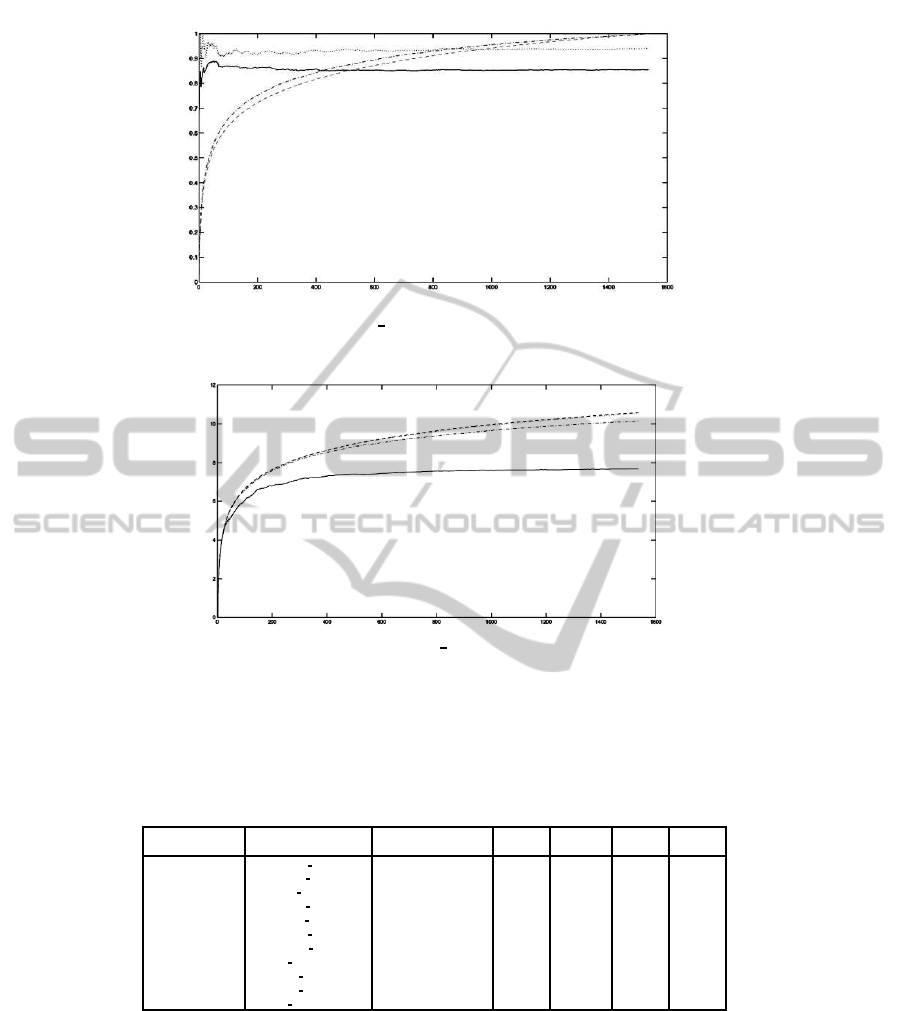
Figure 4: Ocean image and its fastfaded copy (img7 ocean in Table 1): SSIM (solid line), SNR (dotted), SSIM entropy

(increasing dot-line) and SNR entropy (increasing dashed) curves versus the number of blocks.

Figure 5: Ocean image and its Gaussian blurred copy (img57 ocean in Table 1). Entropy versus number of blocks (or an

equivalent number of random pixels). (Bottom-up): SSIM entropy via random pixels (solid) and non overlapping blocks

(dashdot), SNR entropy via random pixels (dotted) and non overlapping blocks (dashed).

Table 1: Images in Fig. 3: Entropy of: the original image (H(X)), the distorted image given the original one (H(Y|X)), SSIM

with overlapping blocks (H(Z)) and SSIM for non overlapping blocks (H(

Z)). For each kind of distortion the parameters used

in LIVE database have been given: the standard deviation of the gaussian kernel for the gaussian blurring, the SNR of the

distortion strength for fastfading, the quality score for jpeg and the standard deviation of the noise distribution for the white

noise. More details in (Sheikh et al., ).

Original Image Distorted Image Distortion kind H(X) H(Y|X) H(Z) H(

ocean img57 ocean Gaussian blur (1.48) 7.1785 4.8630 5.0798 5.3230

stream img58 stream Gaussian blur (3.08) 7.4230 6.6357 5.9525 5.9997

lighthouse img97 lighthouse Gaussian blur (1.48) 7.3799 5.3012 5.1560 5.4239

sailing4 img127 sailing4 Gaussian blur (1.51) 6.8476 5.2000 5.0161 5.1369

ocean img7 ocean fastfading (18.9) 7.1785 4.7998 4.6848 4.8755

house img73 house fastfading (20.3) 7.1803 4.6494 4.0312 4.3385

stream img100 stream jpeg (0.29) 7.4230 6.4137 5.2691 5.5687

ﬂowersonih35 img27 ﬂowersonih35 jpeg (0.93) 7.7161 5.6465 3.4555 3.6996

ocean img118 ocean.bmp white noise (0.035) 7.1785 4.6308 4.2645 4.6762

house img109 house.bmp white noise (0.125) 7.1803 6.4434 6.1604 6.1460

ﬂowersonih35 img72 ﬂowersonih35 white noise (0.070) 7.7161 5.5789 3.6160 3.8698

Selection of the Best Reduction Domain. To test

the results in Section 2.2, the entropy H(X) has been

computed for each image in Fig. 3. Bins width, nec-

essary to build the empirical p.d.f., has been set equal

to 1. With regard to the distorted image J, for each ex-

ample the conditional entropy H(Y|X) has been con-

sidered. The latter has been estimated from H(X−Y),

i.e. by looking at the distortion as an additive term —

even though the process may be much more compli-

cated. However, X −Y really gives the difference of

information between the original image I and the dis-

torted one J. The size of the bin width of H(Y|X)

has been set equal to 1, while 32× 32 blocks have

been used. The entropy H(Z) of the SSIM vector M

has been computed by quantizing M with a bin width

equal to .01. Using these settings, Table 1 shows

that H(Z) < H(X) + H(Y|X). This behavior does not

change for a different setting of parameters. Hence,

SSIM naturally reduces entropy of the original im-

ages.

AFastComputationMethodforIQAMetricsBasedontheirTypicalSet

203

Locality of the Selected Information. Section

2.3 proves that it is more convenient to build FR qual-

ity measure samples using blocks rather than ran-

dom pixels in I and J. Fig. 5 shows that SSIM en-

tropy curve, that has been built using non overlapping

and randomly selected blocks, always assumes val-

ues larger than those of SSIM entropy curve that has

been built using randomly selected pixels. The same

happens for SNR but the effect is strongly less visi-

ble: curves are very close to each other. In all teste,

quantization bins have been set to 10

−4

, even though

different settings conﬁrm the same trend.

Overlapping Blocks. Theoretical results in Sec-

tion 2.4 state that it is more convenient to select non

overlapping blocks from I and J rather than taking

overlapping ones. A simple practical proof has been

made by taking all possible (non overlapping) blocks

from images in Fig. 3 and computing SSIM using

them. Considering a bin width of .01 for this new

vector of measures, the corresponding entropy H(

has been computed. Tests have been performed using

32× 32 blocks. The last column of Table 1 shows that

non overlapping blocks lead to a higher entropy and

then they convey a greater amount of information.

How to ﬁnd a A

Sequence. In order to manually

estimate a sequence belonging to A

, the sequence

size has been ﬁxed and the corresponding error has

been measured. Table 2 contains the results achieved

on Ocean image and its copies distorted by Gaussian

blur, fastfading and white noise. Fig. 6 shows 100

randomly selected 16× 16 blocks that have been used

for the evaluation of SSIM. Both SSIM and SNR have

been considered and the number of samples has been

set equal to 100. On the contrary, the size of the

blocks on I and J has been changed: 8× 8, 16 × 16

and 32× 32. The blocks on I (and the corresponding

in J) have been randomly selected. That’s why the

results in Table 2 have been achieved as average on

30 trials, i.e. 30 different choices of 100 non over-

lapping blocks, in order to get a more fair evaluation

of the estimation error for the considered IQA metric.

Speciﬁcally, the mean and the standard deviation of

the the relative error

M −

(3)

has been computed. For each image and each dis-

tortion kind, the estimation errors always are smaller

than 5% of the true IQA measure. Table 3 contains the

results obtained using different sizes for the selected

sequence of FR values, respectively 50, 100 and 200

blocks on both the original I and the distorted image

J. Again, apart from just one case (in bold) errors are

always under 5%, conﬁrming that few blocks (a little

part of the available information) are required to give

Figure 6: 100 Randomly selected 16× 16 blocks used for

the estimation of SSIM of Ocean image.

a good estimate of the involved FR measure.

The speed up obtained in the computation of the

considered image quality assessment metric on the

typical set depends on the number of blocks that are

used for the evaluation of SSIM. The computational

gain is G =

, where N

is the number of blocks

that are used for the computation of SSIM in the

whole image (using the standard algorithm), while N

is the number of blocks belonging to the visual dis-

tortion typical set i.e, the reduced set of blocks from

which it is possible to get an quite precise estimation

of SSIM. For example, if an image can be partioned

into 1536 non overlapping blocks, the gain using just

50, 100 or 200 non overlapping blocks respectively is

30.72, 15.36 and 7.68. This gain increases if the im-

age is partitioned into non overlapping blocks, while

it decreases for images having small dimension. For

example, for images composed of 1280 non overlap-

ping blocks the gain becomes 27, 13.5 and 6.75 re-

spectively for 50, 100 or 200 non overlapping blocks

in the visual distortion typical set.

4 CONCLUSIONS

The paper has presented a study concerning the def-

inition of a visual distortion typical set in agreement

with the general concept of asymptotic equipartition

property and the neurological studies on those points

that attract human attention in the early vision. Gen-

eral criteria for the characterization and the practical

deﬁnition of this typical set have been given. The typ-

ical set has been used for reducing the amount of in-

formation necessary to assess the quality of an image

using a standard full reference image quality assess-

ment measure. This typical set makes the FR IQA

metric less computational demanding. Achieved re-

sults are very encouraging since they are robust to

changes of image subject, parameters settings and dis-

tortion kinds. Future research will focus on designing

an optimized procedure to ﬁnd the minimum budget

of information for a ﬁxed error.

ICPRAM2014-InternationalConferenceonPatternRecognitionApplicationsandMethods

204

Table 2: Ocean image and its copy distorted by respectively Gaussian blurring (top), fastfading (middle) and white noise

(bottom). Mean and standard deviation (in the brackets) of the relative error (%) for the estimation of the true value of SSIM

and SNR using just 100 blocks with size equal to: 8× 8, 16× 16 and 32× 32.

Block size = 8 /No. Blocks = 100 Block size = 16 /No. Blocks = 100 Block size = 32 /No. Blocks = 100

Total blocks: 6144 Total blocks: 1536 Total blocks: 384

SSIM error SNR error SSIM error SNR error SSIM error SNR error

1.84% (1.41%) 2.46%(2.14%) 1.25%(1.01%) 2.43%(1.63)% 1.40%(1.20%) 2.2% (1.72%)

1.33%(1.42%) 2.75%(2.00%) 1.39%(0.80%) 2.50%(1.90%) 0.79%(0.55%) 2.25%(1.71%)

1.14%(0.87%) 1.31%(1.03%) 1.09%(0.20%) 1.07%(0.70%) 0.71%(0.54%) 0.81%(0.57%)

Table 3: Images in Fig. 3 with different kinds of distortions. Mean value and standard deviation (in brackets) of the relative

error (%) as in eq. (3) for the estimation of the true value of SSIM and SNR considering just 50, 100 and 200 non overlapping

blocks with size equal to 16× 16.

Blk size:16 / Sel. Blks:50 Blk size:16 / Sel. Blks:100 Blk size:16 / Sel. Blks:200

Image Dist Blks SSIM error SNR error SSIM error SNR error SSIM error SNR error

Ocean Gb 1536 2.53% (2.49) 4.15% (2.70) 1.25% (1.01) 2.43% (1.63) 1.16%(1.03) 1.82% (1.18)

Stream Gb 1536 3.50%(3.00) 2.65%(2.25) 3.45%(3.01) 2.29% (1.80) 2.43%(2.01) 1.66%(1.02)

Lighth. Gb 1350 2.45%(2.20) 3.72%(2.01) 2.30%(1.80) 2.39%(2.22) 1.56%(1.21) 1.75%(1.15)

Sail4 Gb 1536 2.13%(2.00) 3.53%(2.99) 1.47%(0.80) 3.26%(2.22) 1.02%(0.45) 1.47%(0.89)

Ocean Ff 1536 1.53% (1.20) 3.18%(2.05) 1.39%(0.80) 2.50%(1.90) 0.83%(0.52) 1.86%(1.01)

House Ff 1536 1.08%(0.99) 2.68%(1.90) 0.75%(0.57) 1.73%(1.60) 0.55%(0.21) 1.36%(0.94)

Stream Jp 1536 2.93%(2.90) 2.78%(2.09) 1.95%(1.50) 1.84%(1.30) 1.56%(0.98) 1.11%(0.80)

Flower Jp 1280 0.58%(0.50) 4.01%(3.03) 0.30%(0.15) 2.62%(2.15) 0.23%(0.09) 1.89%(1.01)

Ocean Wn 1536 1.19%(0.70) 1.29%(0.90) 1.09%(0.80) 1.07%(0.70) 0.61%(0.30) 0.72%(0.31)

House Wn 1536 5.46%(2.09) 2.04%(1.77) 4.40%(2.87%) 1.93%(1.35) 2.72%(2.51) 0.93%(0.80)

Flower Wn 1280 2.82%(2.77) 1.45% (1.35) 1.86%(1.52%) 0.90%(0.50) 1.09%(1.08) 0.56% (0.53)

REFERENCES

Benabdelkader, S. and Boulemden, M. (2005). Recursive

algorithm based on fuzzy 2-partition entropy for 2-

level image thresholding. In Pattern Recognition, 38.

Elsevier.

Bruni, V., Rossi, E., and Vitulano, D. (2013a). Jensen-

shannon divergence for visual quality assessment. In

Signal Image and Video Prcessing 7(3). Springer.

Bruni, V., Vitulano, D., and Ramponi, G. (2011). Image

quality assessment through a subset of the image data.

In Proc. of ISPA 2011. IEEE.

Bruni, V., Vitulano, D., and Wang, Z. (2013b). Special issue

on human vision and information theory. In Signal

Image and Video Prcessing 7(3). Springer.

Cover, T. M. and Thomas, J. A. (1991). Elements of Infor-

mation Theory. John Wiley & sons.

Frazor, R. and Geisler, W. (2006). Local luminance and

contrast in natural in natural images, 46. In Vision

Research.

Gonzalez, R. C. and Woods, R. E. (2002). Digital Image

Processing. Prentice Hall, 2nd edition.

Grunwald, P. D. (2004). A tutorial introduction to the min-

imum description length principle. In Advances in

Minimum Description Length: Theory and Applica-

tions. Myung Grunwald, Pitt,.

Monte, V., Frazor, R., Bonin, V., Geisler, W., and Corandin,

M. (2005). Independence of luminance and contrast

in natural scenes and in the early visual system 8(12).

In Nature Neuroscience.

Rivera, M., Ocegueda, O., and Marroquin, J. L. (2007).

Entropy-controlled quadratic markov measure ﬁeld

models for efﬁcient image segmentation. In IEEE

Trans. on Image Proc. 16(12).

Sheikh, H. R. and Bovik, A. C. (2006). Image information

and visual quality. In IEEE Trans. on Image Proc.,

15(2).

Sheikh, H. R., Bovik, A. C., and Veciana, G. D. (2005). An

information ﬁdelity criterion for image quality assess-

ment using natural scene statistics. In IEEE Trans. on

Image Proc., 14(12).

Sheikh, H. R., Wang, Z., Cormack, L., and

Bovik, A. C. Live image quality assess-

ment database release 2. [Online]. Avail-

able:http://live.ece.utexas.edu/research/quality.

Wang, W., Wang, Y., Huang, Q., and Gao, W. (2010). Mea-

suring visual saliency by site entropy rate. In Proc. of

CVPR10. IEEE.

Wang, Z., Bovik, A. C., Sheikh, H. R., and Simoncelli, E. P.

(2004a). Image quality assessment: From error visi-

bility to structural similarity. In IEEE Trans. on Image

Proc., 13.

Wang, Z. and E.P.Simoncelli (2005). Reduced-reference

image quality assessment using a wavelet-domain nat-

ural image statistic model. In Proc. of Human Vision

and Electronic Imaging X, vol. 5666. SPIE.

Wang, Z. and Li, Q. (2011). Information content weight-

ing for perceptual image quality assessment. In IEEE

Trans. on Image Proc. 20(5).

Wang, Z., Lu, L., and Bovik, A. (2004b). Video quality as-

AFastComputationMethodforIQAMetricsBasedontheirTypicalSet

205

sessment based on structural distortion measurement.

In Signal Processing: Image Communications, 19(2).

Winkler, S. (2005). Digital Video Quality, Vision Models

and Metrics. Wiley.

Zhang, D. and Jernigan, E. (2006). An information theo-

retic criterion for image quality assessment based on

natural scene statistics. In Proc. of ICIP 2006. IEEE.

APPENDIX

Proof 1 1. µ

n+1

− µ

∑

x∈χ

x(p

n+1

(x) − p

(x)) =

∑

x∈χ

−

n+1

(x) +

n+1

− µ

). The sign

of the difference between two successive mean

values depends on x

n+1

and the convergence is

not monotonic. 2. |µ

− µ|

= |

∑

x∈χ

x(p

(x) −

Q(x))|

≤ M

, Q) where V(p

, Q) is the vari-

ational distance between p

and Q i.e., V(p

, Q) =

∑

x∈χ

(x) − Q(x)|. Since the Kullbach-Leibler di-

vergence D

||Q) =

∑

(x)log



(x)

Q(x)



is such

that D

||Q) ≥

, Q), then |µ

− µ|

≤

||Q). Hence, for n: D

||Q) ≤

, ε > 0, then |µ

− µ|

≤ ε•

Proof 3 H(X) = H(α) + αH(X

) + (1 −

α)H(X

) (Cover and Thomas, 1991) and the same

holds for H(Y). Since Z = M(X,Y), then Z =



M(X

) with prob. α

M(X

) with prob. 1− α

where M(X

)

and M(X

) are not disjoint. Z ∼ p

where

= αp

M(X

)

+ (1− α)p

M(X

)

. Hence, H(p

) ≤

H(α) + αH(p

M(X

)

) + (1− α)H(p

M(X

)

). In fact,

let’s suppose that

H(p

) > H(α) + αH(p

M(X

)

) +

+(1− α)H(p

M(X

)

) (4)

and let us consider the Jensen-Shannon

divergence D

M(X

)

||p

M(M(X

)

) =

H(p

) − αH(p

M(X

)

) + (1 − α)H(p

M(X

)

then D

M(X

)

||p

M(X

)

) > H(α), that is

absurd since 0 ≤ D

M(X

)

||p

M(X

)

) ≤

H(α). Since H(p

M(X

)

) ≤ H(p

)

and H(p

M(X

)

) ≤ H(p

)

) we have

H(p

) ≤ H(α) + αH(p

)

) + (1− α)H(p

)

)•

Proof 4 Let

= {Z

, Z

, .., Z

} be a col-

lection of N

variables Z

selected in {Z

, Z

, .., Z

}

and let be K the number of possible N

−ples

such that:

j=1

= {Z

, Z

, .., Z

}. Since for

generic variables S

, .., S

, it holds H(S

, S

, .., S

) ≤

∑

i=1

H(S

), then H(Z

, Z

, .., Z

) ≤

∑

j=1

) ≤

∑

j=1

, ..,

) = KH(

, ..,

) =

,..,

)

•

ICPRAM2014-InternationalConferenceonPatternRecognitionApplicationsandMethods

206