Integrating Local Information-based Link Prediction Algorithms

with OWA Operator

James N. K. Liu

, Yu-Lin He

, Yan-Xing Hu

Xi-Zhao Wang

and Simon C. K. Shiu

Department of Computing, The Hong Kong Polytechnic University, Kowloon, Hong Kong

Key Laboratory in Machine Learning and Computational Intelligence of Hebei Province,

College of Mathematics and Computer Science,Hebei University, Baoding 071002, China

Keywords:

OWA Operator, Link Prediction, Social Network Analysis, Ensemble.

Abstract:

The objective of link prediction for social network is to estimate the likelihood that a link exists between

two nodes x and y. There are some well-known local information-based link prediction algorithms (LILPAs)

which have been proposed to handle this essential and crucial problem in the social network analysis. How-

ever, they can not adequately consider the so-called local information: the degrees of x and y, the number

of common neighbors of nodes x and y, and the degrees of common neighbors of x and y. In other words,

not any LILPA takes into account all the local information simultaneously. This limits the performances of

LILPAs to a certain degree and leads to the high variability of LILPAs. Thus, in order to make full use of

all the local information and obtain a LILPA with highly-predicted capability, an ordered weighted averaging

(OWA) operator based link prediction ensemble algorithm (LPE

OWA

) is proposed by integrating nine different

LILPAs with aggregation weights which are determined with maximum entropy method. The ﬁnal experimen-

tal results on benchmark social network datasets show that LPE

OWA

can obtain higher prediction accuracies

which is measured by the area under the receiver operating characteristic curve (AUC) in comparison with

nine individual LILPAs.

1 INTRODUCTION

With the development of information technology and

big data mining (Lin and Ryaboy, 2013), the social

network analysis is attracting more and more atten-

tions and becoming a research hot-spot of sociology

and statistics. The social network analysis (Carring-

ton et al., 2005; Knoke and Yang, 2008) refers to mine

and discover the underlying knowledge from a so-

cial network diagram by using the mathematical and

graphical techniques. The social network is repre-

sented as a graphic structure that made up of a set

of nodes and links, where nodes represent the indi-

viduals within network and links denote the relation-

ships between individuals. The main studies of so-

cial network analysis include the identiﬁcation of lo-

cal/global patterns, location of social units, and mod-

eling of dynamic network, etc, where the link predic-

tion (Al Hasan and Zaki, 2011; Cukierski et al., 2011;

Dong et al., 2012; Fire et al., 2011; L¨u and Zhou,

2011) as a branch of network pattern recognition is

the most fundamental and essential problem for the

social network analysis.

The link prediction for social network attempts to

estimate the existence likelihood of a link between

two nodes x and y in social network. The essence

of link prediction algorithm is to assign a score for

the non-existent link in social network (L¨u and Zhou,

2011; L¨u et al., 2009; Zhou et al., 2009), where

the score quantiﬁes the existence likelihood of this

non-existent link. So far, there are many link pre-

diction strategies which have been proposed (L¨u and

Zhou, 2011), e.g., similarity-based algorithms, max-

imum likelihood methods, probabilistic models and

so on, where the similarity-based algorithms are most

frequently-usedand simplest ones. Moreover,accord-

ing to the information used to design the measure in-

dices of link existence likelihood, the similarity-based

algorithms can be further classiﬁed into three cate-

gories: local, global and quasi-local ones. In consid-

eration of its easier implementation and less compu-

tational complexity, our tour of studies in this paper

starts with the local information-based link predic-

tion algorithm (LILPA). There are nine representative

LILPAs as follows: common neighbors(CN) (Lorrain

and White, 1971), Salton index (Chowdhury, 2010),

Jaccard index (L¨u and Zhou, 2011), Sφrensen in-

213

Liu J., He Y., Hu Y., Wang X. and Shiu S..

Integrating Local Information-based Link Prediction Algorithms with OWA Operator.

DOI: 10.5220/0004825902130219

In Proceedings of the 3rd International Conference on Pattern Recognition Applications and Methods (ICPRAM-2014), pages 213-219

ISBN: 978-989-758-018-5

 2014 SCITEPRESS (Science and Technology Publications, Lda.)

dex (L¨u and Zhou, 2011), hub promoted index (HPI)

(Ravasz et al., 2002), hub depressed index (HDI)

(L¨u and Zhou, 2011), Leicht-Holme-Newman-I in-

dex (LHN-I) (Leicht et al., 2006), Adamic-Adar index

(AA) (Adamic and Adar, 2003) and resource alloca-

tion index (RA) (Zhou et al., 2009). The comparative

studies (L¨u et al., 2009; Zhao et al., 2012) have re-

ported the merits of LILPAs, but we think there still

exists a defect for the implementations of LILPAs,

i.e., not any LILPA can adequately make use of the

so-called local information (the degrees of x and y, the

number of common neighbors of nodes x and y, and

the degrees of common neighbors of x and y). This

limits the performances (Measured by the area under

the receiver operating characteristic curve (AUC)) of

LILPAs to a certain degree and leads to the higher

variability among LILPAs (Zhang and Ma, 2012).

Inspired by the outlook in L¨u and Zhao’s work (L¨u

and Zhou, 2011), i.e., “we can implement many in-

dividual prediction algorithms and then try to select

and organize them in a proper way. This so-called

ensemble learning method can obtain better predic-

tion performance than could be obtained from any

of the individual algorithms.”, we try to use the en-

semble learning strategy (Zhang and Ma, 2012; Zhou,

2012) to relieve this limitation of LILPAs and accord-

ingly improve the prediction performance of LILPA.

As stated in (Zhang and Ma, 2012), ensemble learning

is such a strategy which is known to reduce the classi-

ﬁers’ variance and improve the decision system’s ro-

bustness and accuracy. The ensembles of some ma-

chine learning algorithms (e.g., decision tree (Ban-

ﬁeld et al., 2007), neural network (Zhou et al., 2002),

support vector machine (Kim et al., 2003), etc.) are

all well and sophisticatedly studied, while there isn’t

any study of ensemble of LILPAs in literatures.

The ordered weighted averaging (OWA) operator

(Yager, 1988) is one of mostly used information ag-

gregation techniques. In view of the effectiveness of

OWA in preference rankings (Wang et al., 2007), an

OWA operator based link prediction ensemble algo-

rithm (LPE

OWA

) is proposed by integrating the nine

above-mentioned LILPAs with aggregation weights

which are determined with maximum entropy method

(O’Hagan, 1988). The experimental results on bench-

mark social networks (Pajek, 2007) demonstrate the

feasibility of our proposed LPE

OWA

and show that

LPE

OWA

can obtain higher prediction accuracies in

comparison with nine individual LILPAs. The rest of

this paper is organized as follows. In Section 2, the

theoretical and empirical analysis to nine LILPAs are

given. In Section 3, the new OWA operator based link

prediction ensemble model (LPE

OWA

) is presented. In

Section 4, experimental comparisonsare conducted to

Table 1: The notation-list.

Notation Meaning

G = hV,Ei A social network graph

A = (a

) The adjacency matrix of G

V The set of nodes in G

E = E

Train

∪ E

Test

The set of links in G (E

Train

∩ E

Test

= Ø)

Train

The training set

Test

The testing set

U The set containing all possible links of G

Predict

= U− E The set containing nonexistent links of G

x ∈ V A node x belonging to V

The existence likelihood of link xy

Γ(x) The set of neighbors of node x

kSk The cardinality of set S

= kΓ(x)k The degree of node x

illustrate the feasibility of proposed ensemble model.

Finally, conclusions are given in Section 5.

2 LILPA ANALYSIS

2.1 Nine Basic LILPAs

For a nonexistent link xy ∈ E

Predict

, LILPAs calculate

the score s

for it to express the likelihood of its ex-

istence. There are nine frequently used LILPAs as

follows. Without loss of generality, we assume there

is no isolated node in G for the sake of simplicity. Our

discussion is based on the notations in Table 1.

• Common neighbors index (CN) (Lorrain and

White, 1971) is the most direct and simplest like-

lihood measure and deﬁned as

= kΓ(x) ∩Γ(y)k. (1)

It is obvious that s





. And, s

repre-

sents the number of paths from x to y with two

steps in G. Thus, the minimum of s

is 0, i.e.,

there is no any path with two steps between x

and y; the maximum of s

is kVk − 2, i.e., all

the residual nodes are served as the intermedi-

ate nodes from x and y. In summary, we get

∈ [0,kVk − 2].

• Salton index (Chowdhury, 2010) considers the de-

grees of nodes and is deﬁned as

Salton

kΓ(x) ∩ Γ(y)k

× k

. (2)

In Eq. (2), k

= kΓ(x)k ∈ [1, kVk − 1] and

= kΓ(y)k ∈ [1, kVk − 1]. Then,

× k

∈

[1, kVk − 1]. Thus, s

Salton

∈ [0, kVk − 2].

ICPRAM2014-InternationalConferenceonPatternRecognitionApplicationsandMethods

214

• Jaccard index (L¨u and Zhou, 2011) is deﬁned as

Jaccard

kΓ(x) ∩ Γ(y)k

kΓ(x) ∪ Γ(y)k

. (3)

Because kΓ(x) ∪ Γ(y)k ∈ [1,kVk], we can derive

Jaccard

∈ [0, kVk − 2].

• Sφrensen index (L¨u and Zhou, 2011) is deﬁned as

Sørensen

2kΓ(x) ∩ Γ(y)k

+ k

. (4)

Because k

+ k

∈ [2, 2(kVk − 1)], we can derive

Sørensen

∈ [0, kVk − 2].

• Hub promoted index (HPI) (Ravasz et al., 2002)

is said to assign a higher score for link connecting

to the nodes with high degrees (Zhao et al., 2012;

Zhou et al., 2009) and deﬁned as

HPI

kΓ(x) ∩ Γ(y)k

min{k

}

∈ [0, kVk − 2]. (5)

• Hub depressed index (HDI) (L¨u and Zhou, 2011)

is opposite to HPI and assigns a lower score for

link connecting to the nodes with high degrees.

The deﬁnition of HDI is

HDI

kΓ(x) ∩ Γ(y)k

max{k

}

∈ [0, kVk − 2]. (6)

• Leicht-Holme-Newman-I index (LHN-I) (Leicht

et al., 2006) is similar to the Salton index and de-

ﬁned as

LHN−I

kΓ(x) ∩ Γ(y)k

× k

∈ [0, kVk − 2]. (7)

The main difference between Salton index and

LHN-I index is the denominator of Eq. (2) and

Eq. (7): the former is

× k

and the latter

× k

. Because k

× k

≥ 1, k

× k

≥

× k

Then, we can get s

Salton

> s

LHNN−I

when k

×k

1. That is to say, for a same link, Salton index al-

ways assigns a higher score compared with LHN-I

index.

• Adamic-Adar index (AA) (Adamic and Adar,

2003) is deﬁned as

∑

z∈Γ(x)∩Γ(y)

log

)

. (8)

Because k

∈ [2,kVk − 1], we can derive s

∈

log

(kVk−1)

,kVk − 2

• Resource allocation index (RA) (Zhou et al.,

2009) is similar to AA index and deﬁned as

∑

z∈Γ(x)∩Γ(y)

∈



kVk − 1

kVk − 2



. (9)

AA and RA indices are all inclined to assign a low

score for the link between x and y which have the

comment neighbors with high degrees. By com-

paring Eq. (8) with Eq. (9), we can ﬁnd s

> s

when Γ(x) ∩ Γ(y) 6= Ø.

2.2 Performance Measure Index-AUC

AUC (L¨u and Zhou, 2011; Zhao et al., 2012) is the

prevalently used index to measure the performance of

link prediction algorithm, which is deﬁned as

AUC =

+ 0.5n

, (10)

where n is the number of independent comparisons

including n

times the missing link having a higher

score, n

times the missing link and nonexistent link

having the same score, and n

times the missing link

having a lower score, i.e., n = n

+ n

. The

missing link denotes the link in testing set E

Test

, and

nonexistent link is the link in E

Predict

. AUC assumes

that a good prediction algorithm is more likely to as-

sign a higher score for the missing link compared with

the nonexistent link.

Assume there are two different link prediction al-

gorithms: AlgoA and AlgoB. If AlgoA obtains a bet-

ter performance, i.e., larger AUC, than AlgoB on the

same E

Test

and E

Predict

, we want to know what con-

clusions can be derived from the result AUC

AlgoA

AUC

AlgoB

From the deﬁnition of Eq. (10), we know

AUC

AlgoA

+ 0.5n

AlgoA

(11)

and

AUC

AlgoB

+ 0.5n

AlgoB

. (12)

Because AUC

AlgoA

> AUC

AlgoB

, we can get

AlgoA

− n

AlgoB

> 0.5



AlgoB

− n

AlgoA



. (13)

As mentioned above, a better link prediction algo-

rithm is assumed to assign a high score for the miss-

ing link in E

Test

more easily. Thus, we think that these

two deductions, i.e, n

AlgoA

= n

AlgoB

, n

AlgoA

> n

AlgoB

AlgoA

< n

AlgoB

and n

AlgoA

< n

AlgoB

, n

AlgoA

> n

AlgoB

AlgoA

< n

AlgoB

, are inadvisable for AUC

AlgoA

AUC

AlgoB

, because n

AlgoA

= n

AlgoB

and n

AlgoA

AlgoB

all deviate from the previous assumption. This

deduction can be demonstrated by the following ex-

perimental results and analysis.

IntegratingLocalInformation-basedLinkPredictionAlgorithmswithOWAOperator

215

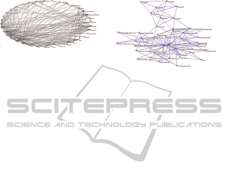
Figure 1: Network of Food Webs-ChesLower.

2.3 High Variability of LILPAs

In this subsection, we study the prediction perfor-

mances of these nine LILPAs. We select two bench-

mark social networks (Pajek, 2007) as shown in Fig. 1

and Fig. 2 for our experimental datasets: Food Webs-

ChesLower and Graph Drawing Contests Data-B97.

The 10-fold cross-validation is used to test the

AUCs of LILPAs. Firstly, the set E including all the

existent links is randomly and averagely divided into

10 disjointed subsets (folds): E = E

∪ E

∪ ··· ∪ E

and E

∩ E

∩ ··· ∩ E

= Ø. Then, we select the sub-

set E

(1 ≤ i ≤ 10) as testing set E

test

in sequence, the

link in which is called missing link. Based on the

test

and kU− Ek, AUC

in Eq. (10) is calculated

for ith fold dataset. Finally, 10 AUCs on 10 folds are

averaged as the evaluation result of link prediction al-

gorithm. The detailed experimental results on these

two networks are summarized in Table 2 and Table 3

respectively. By observing the experimental results,

we can get the following conclusions:

• According to the prediction performance, we can

divide the above-mentioned 9 LILPAs into three

categories: AA and RA obtain the higher AUCs,

CN the medium AUC and other 6 algorithms the

lowerAUCs. From Eqs. (1)-(9), we knowthat AA

and RA consider the degrees of common neigh-

bors of x and y, CN considers the number of com-

mon neighbors of x and y, and other algorithms

consider the number of common neighbors of x

and y and the degrees of x and y synchronously

(The item kΓ(x) ∪ Γ(y)k in Jaccard index equals

to k

+ k

when there are no common neighbors

for x and y).

• For the different link prediction algorithms Al-

goA and AlgoB, when AUC

AlgoA

> AUC

AlgoB

we can get n

AlgoA

> n

AlgoB

. E.g., from the ex-

perimental results in Tables 2 and 3, we can ﬁnd

that under the situation of AUC

> AUC

(ChesLower) = 6038 > n

(ChesLower) =

5424 and n

(B97) = 19998 > n

(B97) =

17399 hold for the employed two networks re-

spectively. This empirical conclusion also reﬂects

Figure 2: Network of Graph Drawing Contests Data-B97.

that increasing the number of missing links having

higher scores is the key for improving the perfor-

mance of LILPA from another perspective.

• The variability of LILPAs is high. We can ﬁnd

that the prediction performances of different LIL-

PAs are varying dramatically for the same train-

ing and testing datasets. For example, n

=5110,

4083, 4254, 4254, 3263, 4444, 1846, 5620 and

5791 respectively on the Fold 5 of ChesLower and

=16892, 16273, 15567, 15567, 17280, 15147,

14605, 19606 and 19977 respectively on the Fold

9 of B97.

From the foregoing analysis, we can ﬁnd that no

any link prediction algorithm mentioned in Subsec-

tion 2.1 can consider the degrees of x and y, the com-

mon neighbors of x and y, and the degrees of common

neighbors of x and y simultaneously. This leads to the

high variability of LILPAs and limits the prediction

performances of LILPAs.

3 LPE

OWA

ALGORITHM

The n-dimensional OWA operator is a mapping F :

ℜ

→ ℜ with an associated weight vector ~w =

,··· , w

) such that

∑

i=1

= 1, w

∈ [0,1],i = 1,2, ··· , n (14)

and

F(a

,··· , a

) =

∑

i=1

, (15)

where b

is the ith largest value of a

,··· , a

. The

important issue of applying OWA operator is deter-

mining the weight vector ~w of OWA operator.

In order to determine the weight vector ~w, two

important measures Disp(~w) and orness(~w) are de-

ﬁned, where Disp(~w) measures the degree to which all

ICPRAM2014-InternationalConferenceonPatternRecognitionApplicationsandMethods

216

Table 2: Prediction performances of nine LILPAs on the network of Food Webs-ChesLower.

Fold 1 Fold 2 Fold 3 Fold 4 Fold 5 Fold 6 Fold 7 Fold 8 Fold 9 Fold 10 Average

CN [4326 1143 3014 0.5773] [5686 956 1841 0.7266] [5164 731 2588 0.6518] [5926 1038 1519 0.7598] [6170 761 1552 0.7722] [5110 785 2588 0.6487] [4833 1155 2495 0.6378] [4733 943 2308 0.6519] [6850 456 678 0.8865] [5441 695 1848 0.7250] [5424 866 2043 0.7038±0.0079]

Salton [3111 60 5312 0.3703] [4134 47 4302 0.4901] [3474 31 4978 0.4114] [3805 47 4631 0.4513] [4675 51 3757 0.5541] [4083 24 4376 0.4827] [3574 20 4889 0.4225] [3551 23 4410 0.4462] [5364 19 2601 0.6730] [4273 16 3695 0.5362] [4004 34 4295 0.4838±0.0075]

Jaccard [3063 143 5277 0.3695] [4134 140 4209 0.4956] [3380 99 5004 0.4043] [3688 216 4579 0.4475] [4605 110 3768 0.5493] [4254 142 4087 0.5098] [3362 260 4861 0.4116] [3335 61 4588 0.4215] [5117 101 2766 0.6472] [4254 151 3579 0.5423] [3919 142 4272 0.4799±0.0072]

Sφrensen [3063 143 5277 0.3695] [4134 140 4209 0.4956] [3380 99 5004 0.4043] [3688 216 4579 0.4475] [4605 110 3768 0.5493] [4254 142 4087 0.5098] [3362 260 4861 0.4116] [3335 61 4588 0.4215] [5117 101 2766 0.6472] [4254 151 3579 0.5423] [3919 142 4272 0.4799±0.0072]

HPI [2596 688 5199 0.3466] [3734 472 4277 0.4680] [3747 210 4526 0.4541] [3564 633 4286 0.4574] [4257 716 3510 0.5440] [3263 480 4740 0.4129] [3966 508 4009 0.4975] [3799 633 3552 0.5155] [5200 502 2282 0.6827] [3472 467 4045 0.4641] [3760 531 4043 0.4843±0.0078]

HDI [3271 215 4997 0.3983] [4184 208 4091 0.5055] [3245 164 5074 0.3922] [3763 169 4551 0.4536] [4521 150 3812 0.5418] [4444 164 3875 0.5335] [3291 123 5069 0.3952] [3168 100 4716 0.4031] [4885 87 3012 0.6173] [4445 102 3437 0.5631] [3922 148 4263 0.4804±0.0068]

LHN-I [1524 125 6834 0.1870] [2023 116 6344 0.2453] [1218 90 7175 0.1489] [1170 57 7256 0.1413] [2137 172 6174 0.2621] [1846 84 6553 0.2226] [1624 54 6805 0.1946] [1193 44 6747 0.1522] [1959 88 5937 0.2509] [1751 48 6185 0.2223] [1645 88 6601 0.2027±0.0020]

AA [5042 157 3284 0.6036] [6434 59 1990 0.7619] [5684 65 2734 0.6739] [6883 4 1596 0.8116] [6645 71 1767 0.7875] [5620 102 2761 0.6685] [5522 243 2718 0.6653] [5446 187 2351 0.6938] [7209 3 772 0.9031] [5899 28 2057 0.7406] [6038 92 2203 0.7310±0.0077]

RA [5001 157 3325 0.5988] [6465 59 1959 0.7656] [5714 65 2704 0.6774] [6995 4 1484 0.8248] [6773 71 1639 0.8026] [5791 102 2590 0.6887] [5596 243 2644 0.6740] [5596 187 2201 0.7126] [7221 3 760 0.9046] [5915 28 2041 0.7426] [6107 92 2135 0.7392±0.0078]

Note: The quadruple denotes [n

AUC].

Table 3: Prediction performances of nine LILPAs on the network of Graph Drawing Contests Data-B97.

Fold 1 Fold 2 Fold 3 Fold 4 Fold 5 Fold 6 Fold 7 Fold 8 Fold 9 Fold 10 Average

CN [18250 3946 2185 0.8295] [18159 3946 2276 0.8257] [19026 3607 1748 0.8543] [15959 5113 3309 0.7594] [17751 3711 2016 0.8351] [16210 4297 2971 0.7819] [16484 4271 2723 0.7931] [18148 3511 1819 0.8478] [16892 4141 2445 0.8077] [17113 3879 2486 0.8115] [17399 4042 2398 0.8146±0.0009]

Salton [17065 223 7093 0.7045] [17203 248 6930 0.7107] [17945 161 6275 0.7393] [15190 1018 8173 0.6439] [17374 271 5833 0.7458] [15518 1050 6910 0.6833] [15748 624 7106 0.6840] [16720 204 6554 0.7165] [16273 227 6978 0.6980] [16970 652 5856 0.7367] [16601 468 6771 0.7063±0.0010]

Jaccard [16294 354 7733 0.6756] [16341 443 7597 0.6793] [17040 351 6990 0.7061] [14396 1286 8699 0.6168] [17104 481 5893 0.7388] [15121 1261 7096 0.6709] [15213 751 7514 0.6640] [15803 300 7375 0.6795] [15567 414 7497 0.6719] [16709 757 6012 0.7278] [15959 640 7241 0.6831±0.0012]

Sφrensen [16294 354 7733 0.6756] [16341 443 7597 0.6793] [17040 351 6990 0.7061] [14396 1286 8699 0.6168] [17104 481 5893 0.7388] [15121 1261 7096 0.6709] [15213 751 7514 0.6640] [15803 300 7375 0.6795] [15567 414 7497 0.6719] [16709 757 6012 0.7278] [15959 640 7241 0.6831±0.0012]

HPI [18458 1481 4442 0.7874] [18383 2055 3943 0.7961] [18793 1969 3619 0.8112] [16581 2990 4810 0.7414] [17184 2051 4243 0.7756] [15561 2729 5188 0.7209] [17023 2429 4026 0.7768] [18485 1897 3096 0.8277] [17280 1723 4475 0.7727] [16666 2420 4392 0.7614] [17441 2174 4223 0.7771±0.0010]

HDI [15793 590 7998 0.6599] [15738 608 8035 0.6580] [16371 507 7503 0.6819] [14037 1299 9045 0.6024] [16619 591 6268 0.7204] [14774 1223 7481 0.6553] [14845 757 7876 0.6484] [15018 344 8116 0.6470] [15147 469 7862 0.6551] [16224 970 6284 0.7117] [15457 736 7647 0.6640±0.0011]

LHN-I [14940 276 9165 0.6184] [14999 340 9042 0.6222] [15477 269 8635 0.6403] [13617 1050 9714 0.5800] [15198 390 7890 0.6556] [13769 1057 8652 0.6090] [14049 626 8803 0.6117] [14360 218 8900 0.6163] [14605 294 8579 0.6283] [14948 756 7774 0.6528] [14596 528 8715 0.6235±0.0005]

AA [20839 324 3218 0.8614] [20981 325 3075 0.8672] [21986 174 2221 0.9053] [18965 1211 4205 0.8027] [20709 206 2563 0.8864] [18414 1247 3817 0.8109] [19291 746 3441 0.8376] [20138 409 2931 0.8664] [19606 507 3365 0.8459] [19047 931 3500 0.8311] [19998 608 3234 0.8515±0.0010]

RA [21010 323 3048 0.8684] [21352 325 2704 0.8824] [22149 174 2058 0.9120] [19257 1211 3913 0.8147] [20941 206 2331 0.8963] [18764 1247 3467 0.8258] [19585 745 3148 0.8501] [20026 409 3043 0.8617] [19977 507 2994 0.8617] [19169 931 3378 0.8363] [20223 608 3008 0.8609±0.0009]

the aggregates are equally used and orness(~w) mea-

sures the degree to which the aggregation is like an

or operation. O’Hagan’s maximum entropy method

(O’Hagan, 1988) is one of the commonly used meth-

ods for determining the weight vector of OWA oper-

ator, which solves ~w from the following constrained

nonlinear optimization model:

Maximize Disp(~w) = −

∑

i=1

In(w

)

s.t. orness(~w) = α =

n−1

∑

i=1

(n− i)w

∑

i=1

= 1,

∈ [0,1],i = 1, 2, · ·· , n,

(16)

where α ∈ [0, 1] is the optimism level factor, which

controls the desired degree of orness. When

α = 0, ~w = (0, ··· ,0,1) and F(a

,··· , a

) = b

= min{a

}; when α = 1, ~w = (1, 0,··· , 0) and

F(a

,··· , a

) = b

= max{a

}; when α = 0.5, ~w =



,··· ,



and F(a

,··· , a

) =

∑

i=1

∑

i=1

LINGO software is used to ﬁnd the optimized weight

vector ~w for Eq. (16). In this study, because OWA op-

erator will be used to aggregate 9 different LILPAs,

we let n = 9 in the following implementation.

LPE

OWA

is such an ensemble algorithm which in-

tegrates 9 LILPAs with OWA operator to carry out

the link prediction for social network. The likelihood

score of a link existence calculated with LPE

OWA

deﬁned as follows:

OWA

∑

i=1

(i)

, (17)

where s

(i)

∈ [0,1] is the ith largest value of sn

Salton

, sn

Jaccard

, sn

Sørensen

, sn

HPI

, sn

HDI

, sn

LHN−I

and sn

which are the normalization of s

Salton

, s

Jaccard

, s

Sørensen

, s

HPI

, s

HDI

, s

LHN−I

, s

and

as shown in Eqs. (1)-(9), w

(i = 1, 2, ··· , 9) is the

weight of OWA operator, which is determined with

maximum entropy method.

The role of normalization is to locate the likeli-

hood scores in the interval [0,1] and regards the like-

lihood score as a probability value. For the k

> 2

and k

6= k

, we can derive

1 < min{k

} <

+ k

< max{k

} < kΓ(x) ∪ Γ(y)k < k

(18)

Furthermore, we can get the following derivations:

> s

HPI

> s

Salton

> s

Sørensen

> s

HDI

> s

Jaccard

> s

LHN−I

(19)

and

> sn

HPI

> sn

Salton

> sn

Sørensen

> sn

HDI

> sn

Jaccard

> sn

LHN−I

(20)

For any node z ∈ kΓ(x) ∩ Γ(y)k, when k

> 2, we

can obtain

1 < log

< k

⇒ 1 >

log

. (21)

Considering s

= kΓ(x) ∩ Γ(y)k =

∑

z∈kΓ(x)∩Γ(y)k

we can derive

> s

and sn

> sn

. (22)

Eqs. (20) and (22) tell us that the individual algo-

rithm only considers the number of common neigh-

bors of two different nodes x and y, to obtain the high-

est weight in LPE

OWA

, because it is obvious and direct

that a link will more likely exist between two nodes

x and y if they have more common neighbors. This

kind of local information plays a more crucial role in

the link prediction compared with other two local in-

formation, i.e., the degrees of x and y and the degrees

of common neighbors of x and y.

IntegratingLocalInformation-basedLinkPredictionAlgorithmswithOWAOperator

217

Table 4: Prediction performances of LPE

OWA

on the network of Food Webs-ChesLowerl.

orness(~w) = α Fold 1 Fold 2 Fold 3 Fold 4 Fold 5 Fold 6 Fold 7 Fold 8 Fold 9 Fold 10 Average

0.55 [5362 30 3091 0.6339] [6586 13 1884 0.7771] [5796 19 2668 0.6844] [7217 3 1263 0.8509] [6842 15 1626 0.8074] [5868 64 2551 0.6955] [5750 78 2655 0.6824] [5842 90 2052 0.7373] [7244 1 739 0.9074] [5968 9 2007 0.7481] [6248 32 2054 0.7524±0.0072]

0.60 [5470 30 2983 0.6466] [6601 13 1869 0.7789] [5802 19 2662 0.6851] [7373 3 1107 0.8693] [6832 15 1636 0.8063] [5867 64 2552 0.6954] [5799 78 2606 0.6882] [5973 90 1921 0.7538] [7242 1 741 0.9071] [5979 9 1996 0.7494] [6294 32 2007 0.7580±0.0071]

0.65 [5571 30 2882 0.6585] [6620 13 1850 0.7812] [5814 19 2650 0.6865] [7462 3 1018 0.8798] [6824 15 1644 0.8053] [5860 64 2559 0.6946] [5903 78 2502 0.7005] [6086 90 1808 0.7679] [7227 1 756 0.9052] [5972 9 2003 0.7486] [6334 32 1967 0.7628±0.0068]

0.70 [5658 30 2795 0.6687] [6647 13 1823 0.7843] [5846 19 2618 0.6903] [7505 3 975 0.8849] [6830 15 1638 0.8060] [5857 64 2562 0.6942] [6012 78 2393 0.7133] [6168 90 1726 0.7782] [7225 1 758 0.9050] [5979 9 1996 0.7494] [6373 32 1928 0.7674±0.0065]

0.75 [5681 30 2772 0.6715] [6641 13 1829 0.7836] [5845 19 2619 0.6901] [7549 3 931 0.8901] [6780 15 1688 0.8001] [5837 64 2582 0.6919] [6062 78 2343 0.7192] [6236 90 1658 0.7867] [7229 1 754 0.9055] [5947 9 2028 0.7454] [6381 32 1920 0.7684±0.0066]

0.80 [5705 30 2748 0.6743] [6660 13 1810 0.7859] [5869 19 2595 0.6930] [7577 3 903 0.8934] [6743 15 1725 0.7958] [5832 64 2587 0.6913] [6107 78 2298 0.7245] [6270 90 1624 0.7910] [7217 1 766 0.9040] [5925 9 2050 0.7427] [6391 32 1911 0.7696±0.0065]

0.85 [5745 30 2708 0.6790] [6705 13 1765 0.7912] [5915 19 2549 0.6984] [7599 3 881 0.8960] [6743 15 1725 0.7958] [5798 64 2621 0.6873] [6144 78 2261 0.7289] [6306 90 1588 0.7955] [7205 1 778 0.9025] [5924 9 2051 0.7425] [6408 32 1893 0.7717±0.0064]

0.90 [5766 30 2687 0.6815] [6741 13 1729 0.7954] [5949 19 2515 0.7024] [7610 3 870 0.8973] [6716 15 1752 0.7926] [5795 64 2624 0.6869] [6183 78 2222 0.7335] [6341 90 1553 0.7998] [7200 1 783 0.9019] [5893 9 2082 0.7387] [6419 32 1882 0.7730±0.0064]

0.92 [5769 30 2684 0.6818] [6743 13 1727 0.7957] [5955 19 2509 0.7031] [7613 3 867 0.8976] [6701 15 1767 0.7908] [5799 64 2620 0.6874] [6193 78 2212 0.7346] [6345 90 1549 0.8004] [7196 1 787 0.9014] [5877 9 2098 0.7367] [6419 32 1882 0.7729±0.0063]

0.93 [5770 30 2683 0.6820] [6758 13 1712 0.7974] [5968 19 2496 0.7046] [7618 3 862 0.8982] [6701 15 1767 0.7908] [5800 64 2619 0.6875] [6196 78 2209 0.7350] [6347 90 1547 0.8006] [7196 1 787 0.9014] [5877 9 2098 0.7367] [6423 32 1878 0.7734±0.0063]

0.94 [5770 30 2683 0.6820] [6757 13 1713 0.7973] [5969 19 2495 0.7048] [7625 3 855 0.8990] [6693 15 1775 0.7899] [5801 64 2618 0.6876] [6200 78 2205 0.7355] [6350 90 1544 0.8010] [7196 1 787 0.9014] [5865 9 2110 0.7352] [6423 32 1879 0.7734±0.0063]

0.95 [5772 30 2681 0.6822] [6758 13 1712 0.7974] [5971 19 2493 0.7050] [7628 3 852 0.8994] [6686 15 1782 0.7890] [5801 64 2618 0.6876] [6194 78 2211 0.7348] [6353 90 1541 0.8014] [7196 1 787 0.9014] [5859 9 2116 0.7344] [6422 32 1879 0.7733±0.0064]

0.96 [5773 30 2680 0.6823] [6760 13 1710 0.7977] [5973 19 2491 0.7052] [7634 3 846 0.9001] [6686 15 1782 0.7890] [5797 64 2622 0.6871] [6199 78 2206 0.7354] [6360 90 1534 0.8022] [7194 1 789 0.9011] [5859 9 2116 0.7344] [6424 32 1878 0.7735±0.0064]

0.97 [5773 30 2680 0.6823] [6768 13 1702 0.7986] [5982 19 2482 0.7063] [7642 3 838 0.9010] [6673 15 1795 0.7875] [5796 64 2623 0.6870] [6201 78 2204 0.7356] [6363 90 1531 0.8026] [7188 1 795 0.9004] [5859 9 2116 0.7344] [6425 32 1877 0.7736±0.0064]

0.98 [5773 30 2680 0.6823] [6769 13 1701 0.7987] [5983 19 2481 0.7064] [7642 3 838 0.9010] [6673 15 1795 0.7875] [5796 64 2623 0.6870] [6202 78 2203 0.7357] [6363 90 1531 0.8026] [7188 1 795 0.9004] [5859 9 2116 0.7344] [6425 32 1876 0.7736±0.0064]

Table 5: Prediction performances of LPE

OWA

on the network of Graph Drawing Contests Data-B97.

orness(~w) = α Fold 1 Fold 2 Fold 3 Fold 4 Fold 5 Fold 6 Fold 7 Fold 8 Fold 9 Fold 10 Average

0.55 [20852 148 3381 0.8583] [19275 1351 3755 0.8183] [20854 123 3404 0.8579] [21653 71 2657 0.8896] [20137 195 3146 0.8618] [20822 79 2577 0.8886] [20665 509 2304 0.8910] [19633 891 2954 0.8552] [20958 136 2384 0.8956] [21101 69 2308 0.9002] [20595 357 2887 0.8716±0.0007]

0.60 [20894 148 3339 0.8600] [19385 1351 3645 0.8228] [21057 123 3201 0.8662] [21749 71 2561 0.8935] [20253 195 3030 0.8668] [21032 79 2367 0.8975] [20748 508 2222 0.8945] [19662 891 2925 0.8564] [21044 136 2298 0.8992] [21246 68 2164 0.9064] [20707 357 2775 0.8763±0.0007]

0.65 [20923 148 3310 0.8612] [19449 1351 3581 0.8254] [21169 123 3089 0.8708] [21839 71 2471 0.8972] [20307 195 2976 0.8691] [21161 79 2238 0.9030] [20784 508 2186 0.8961] [19684 891 2903 0.8574] [21073 136 2269 0.9005] [21343 68 2067 0.9105] [20773 357 2709 0.8791±0.0007]

0.70 [21011 148 3222 0.8648] [19516 1351 3514 0.8282] [21263 123 2995 0.8746] [21880 71 2430 0.8989] [20385 195 2898 0.8724] [21249 79 2150 0.9067] [20814 508 2156 0.8974] [19678 891 2909 0.8571] [21088 136 2254 0.9011] [21380 68 2030 0.9121] [20826 357 2656 0.8813±0.0007]

0.75 [21035 148 3198 0.8658] [19584 1351 3446 0.8310] [21349 123 2909 0.8782] [22002 71 2308 0.9039] [20426 195 2857 0.8742] [21374 79 2025 0.9121] [20838 508 2132 0.8984] [19709 891 2878 0.8584] [21158 136 2184 0.9041] [21439 68 1971 0.9146] [20891 357 2591 0.8841±0.0007]

0.80 [21164 148 3069 0.8711] [19625 1351 3405 0.8326] [21369 123 2889 0.8790] [22104 71 2206 0.9081] [20496 195 2787 0.8771] [21415 79 1984 0.9138] [20874 508 2096 0.8999] [19717 891 2870 0.8588] [21194 136 2148 0.9056] [21492 68 1918 0.9169] [20945 357 2537 0.8863±0.0007]

0.85 [21240 148 2993 0.8742] [19621 1351 3409 0.8325] [21411 123 2847 0.8807] [22164 71 2146 0.9105] [20559 195 2724 0.8798] [21433 79 1966 0.9146] [20921 508 2049 0.9019] [19715 891 2872 0.8587] [21210 136 2132 0.9063] [21542 68 1868 0.9190] [20982 357 2501 0.8878±0.0008]

0.90 [21314 148 2919 0.8772] [19624 1351 3406 0.8326] [21446 123 2812 0.8821] [22242 71 2068 0.9137] [20625 195 2658 0.8826] [21414 79 1985 0.9138] [20972 508 1998 0.9041] [19689 891 2898 0.8576] [21222 136 2120 0.9068] [21610 68 1800 0.9219] [21016 357 2466 0.8892±0.0008]

0.92 [21325 148 2908 0.8777] [19632 1351 3398 0.8329] [21457 123 2801 0.8826] [22261 71 2049 0.9145] [20641 195 2642 0.8833] [21426 79 1973 0.9143] [20989 508 1981 0.9048] [19735 891 2852 0.8595] [21275 136 2067 0.9091] [21619 68 1791 0.9223] [21036 357 2446 0.8901±0.0008]

0.93 [21318 148 2915 0.8774] [19632 1351 3398 0.8329] [21468 123 2790 0.8830] [22277 71 2033 0.9152] [20669 195 2614 0.8845] [21431 79 1968 0.9145] [21002 508 1968 0.9054] [19743 891 2844 0.8599] [21296 136 2046 0.9100] [21628 68 1782 0.9227] [21046 357 2436 0.8905±0.0008]

0.94 [21318 148 2915 0.8774] [19633 1351 3397 0.8330] [21477 123 2781 0.8834] [22283 71 2027 0.9154] [20678 195 2605 0.8849] [21427 79 1972 0.9143] [21005 508 1965 0.9055] [19750 891 2837 0.8602] [21305 136 2037 0.9103] [21638 68 1772 0.9231] [21051 357 2431 0.8907±0.0008]

0.95 [21317 148 2916 0.8774] [19629 1351 3401 0.8328] [21479 123 2779 0.8835] [22272 71 2038 0.9150] [20675 195 2608 0.8848] [21415 79 1984 0.9138] [21007 509 1962 0.9056] [19741 891 2846 0.8598] [21304 136 2038 0.9103] [21645 69 1764 0.9234] [21048 357 2434 0.8906±0.0008]

0.96 [21330 148 2903 0.8779] [19631 1351 3399 0.8329] [21483 123 2775 0.8837] [22279 71 2031 0.9152] [20679 195 2604 0.8849] [21421 79 1978 0.9141] [21007 509 1962 0.9056] [19748 891 2839 0.8601] [21311 136 2031 0.9106] [21655 69 1754 0.9238] [21054 357 2428 0.8909±0.0008]

0.97 [21331 148 2902 0.8779] [19633 1351 3397 0.8330] [21489 123 2769 0.8839] [22280 71 2030 0.9153] [20686 195 2597 0.8852] [21426 79 1973 0.9143] [21008 508 1962 0.9056] [19759 891 2828 0.8606] [21322 136 2020 0.9111] [21666 68 1744 0.9243] [21060 357 2422 0.8911±0.0008]

0.98 [21335 148 2898 0.8781] [19633 1351 3397 0.8330] [21489 123 2769 0.8839] [22282 71 2028 0.9154] [20686 195 2597 0.8852] [21426 79 1973 0.9143] [21008 508 1962 0.9056] [19759 891 2828 0.8606] [21322 136 2020 0.9111] [21668 68 1742 0.9244] [21061 357 2421 0.8911±0.0008]

4 EXPERIMENTATION

The prediction performance of LPE

OWA

is also tested

on the social networks of ChesLower and B97. We

compare LPE

OWA

with other 9 LILPAs on the same

folds. 15 differentvalues are assigned to the optimism

level factor α. The detailed experimental results are

summarized in Table 4 and Table 5.

Three advantages of LPE

OWA

can be found by

observing these experimental results: (1) LPE

OWA

obtains higher prediction accuracies compared with

any individual LILPA through increasing the numbers

of individual missing links (i.e., n

s) having higher

scores. For example, n

s on any fold in Table 4 and

Table 5 are larger than the corresponding ones in Ta-

ble 2 and Table 3. (2) LPE

OWA

reduces the possibility

that user selects a weak LILPA and thus improve the

high variability of LILPAs. (3) LPE

OWA

is more sta-

ble in comparison with individual LILPAs because of

the lower prediction variances in Table 4 and Table 5.

In addition, the computational complexity of LPE

OWA

is O(kVk) which is same as the individual LILPAs.

The selection of parameter α plays a positive impact

on the performance of LPE

OWA

, i.e., the larger α gives

rise to higher prediction accuracy by emphasizing the

individual LILPA with higher probability.

We think the better performances of LPE

OWA

are

derived from the adequate utilization of the local in-

formation. Besides the more direct number of com-

mon neighbors of x and y, LPE

OWA

also considers the

degrees of x and y and the degrees of common neigh-

bors of x and y.

5 CONCLUSIONS

This paper studies the ensemble problem of link pre-

diction algorithm for the ﬁrst time. An OWA oper-

ator based ensemble strategy LPE

OWA

for integrat-

ing nine local information-based link prediction algo-

rithms is proposed. The feasibility and effectiveness

of LPE

OWA

are demonstrated by the experimental re-

sults on benchmark social networks. A number of en-

hancements and future research can be summarized

as follows: (1) testing the performance of LPE

OWA

on the social networks with millions of nodes col-

lected from well-known social-networking sites, e.g.,

Flickr, Facebook, Weibo and etc; (2) developing the

optimization mechanism for the selection of optimism

level factor α; and (3) comparing LPE

OWA

with other

aggregation/ensemble strategies.

ACKNOWLEDGEMENTS

This work was supported in part by the CRG grants G-

YL14 and G-YM07 of The Hong Kong Polytechnic

University and by the National Natural Science Foun-

dations of China under Grant 61170040 and Grant

71371063.

REFERENCES

Adamic, L. A. and Adar, E. (2003). Friends and neighbors

on the web. Social Networks, 25(3):211–230.

Al Hasan, M. and Zaki, M. J. (2011). A survey of link

ICPRAM2014-InternationalConferenceonPatternRecognitionApplicationsandMethods

218

prediction in social networks. In Social Network Data

Analytics, pages 243–275. Springer.

Banﬁeld, R. E., Hall, L. O., Bowyer, K. W., and

Kegelmeyer, W. P. (2007). A comparison of deci-

sion tree ensemble creation techniques. Pattern Anal-

ysis and Machine Intelligence, IEEE Transactions on,

29(1):173–180.

Carrington, P. J., Scott, J., and Wasserman, S. (2005). Mod-

els and methods in social network analysis. Cam-

bridge University Press.

Chowdhury, G. (2010). Introduction to modern information

retrieval. Facet Publishing.

Cukierski, W., Hamner, B., and Yang, B. (2011). Graph-

based features for supervised link prediction. In Neu-

ral Networks (IJCNN), The 2011 International Joint

Conference on, pages 1237–1244. IEEE.

Dong, Y., Tang, J., Wu, S., Tian, J., Chawla, N. V., Rao,

J., and Cao, H. (2012). Link prediction and recom-

mendation across heterogeneous social networks. In

Data Mining (ICDM), 2012 IEEE 12th International

Conference on, pages 181–190. IEEE.

Fire, M., Tenenboim, L., Lesser, O., Puzis, R., Rokach, L.,

and Elovici, Y. (2011). Link prediction in social net-

works using computationally efﬁcient topological fea-

tures. In Privacy, Security, Risk and Trust (PASSAT),

2011 IEEE Third International Conference on and So-

cial Computing (SOCIALCOM), 2011 IEEE Third In-

ternational Conference on, pages 73–80. IEEE.

Kim, H.-C., Pang, S., Je, H.-M., Kim, D., and Yang Bang,

S. (2003). Constructing support vector machine en-

semble. Pattern Recognition, 36(12):2757–2767.

Knoke, D. and Yang, S. (2008). Social network analysis,

volume 154. Sage.

Leicht, E., Holme, P., and Newman, M. (2006). Vertex sim-

ilarity in networks. Physical Review E, 73(2):026120.

Lin, J. and Ryaboy, D. (2013). Scaling big data mining

infrastructure: the twitter experience. ACM SIGKDD

Explorations Newsletter, 14(2):6–19.

Lorrain, F. and White, H. C. (1971). Structural equiva-

lence of individuals in social networks. The Journal

of Mathematical Sociology, 1(1):49–80.

L¨u, L., Jin, C.-H., and Zhou, T. (2009). Similarity index

based on local paths for link prediction of complex

networks. Physical Review E, 80(4):046122.

L¨u, L. and Zhou, T. (2011). Link prediction in complex

networks: A survey. Physica A: Statistical Mechanics

and its Applications, 390(6):1150–1170.

O’Hagan, M. (1988). Aggregating template or rule an-

tecedents in real-time expert systems with fuzzy set

logic. In Signals, Systems and Computers, Twenty-

Second Asilomar Conference on, volume 2, pages

681–689. IEEE.

Pajek (2007). http://vlado.fmf.uni-lj.si/pub/networks/data/.

Ravasz, E., Somera, A. L., Mongru, D. A., Oltvai, Z. N.,

and Barab´asi, A.-L. (2002). Hierarchical organiza-

tion of modularity in metabolic networks. Science,

297(5586):1551–1555.

Wang, Y.-M., Luo, Y., and Hua, Z. (2007). Aggregating

preference rankings using owa operator weights. In-

formation Sciences, 177(16):3356–3363.

Yager, R. R. (1988). On ordered weighted averaging aggre-

gation operators in multicriteria decisionmaking. Sys-

tems, Man and Cybernetics, IEEE Transactions on,

18(1):183–190.

Zhang, C. and Ma, Y. (2012). Ensemble machine learning:

methods and applications. Springer.

Zhao, J., Feng, X., Dong, L., Liang, X., and Xu, K. (2012).

Performance of local information-based link predic-

tion: a sampling perspective. Journal of Physics A:

Mathematical and Theoretical, 45(34):345001.

Zhou, T., L¨u, L., and Zhang, Y.-C. (2009). Predicting miss-

ing links via local information. The European Physi-

cal Journal B, 71(4):623–630.

Zhou, Z.-H. (2012). Ensemble methods: foundations and

algorithms. CRC Press.

Zhou, Z.-H., Wu, J., and Tang, W. (2002). Ensembling neu-

ral networks: many could be better than all. Artiﬁcial

Intelligence, 137(1):239–263.

IntegratingLocalInformation-basedLinkPredictionAlgorithmswithOWAOperator

219