Data Cube Computational Model with Hadoop MapReduce

Bo Wang

, Hao Gui

, Mark Roantree

and Martin F. O’Connor

International School of Software, Wuhan University, Wuhan, China

Insight: Centre for Data Analytics, Dublin City University, Dublin, Ireland

Keywords:

XML, Hadoop, Data Warehouse, MapReduce.

Abstract:

XML has become a widely used and well structured data format for digital document handling and message

transmission. To ﬁnd useful knowledge in XML data, data warehouse and OLAP applications aimed at pro-

viding supports for decision making should be developed. Apache Hadoop is an open source cloud computing

framework that provides a distributed ﬁle system for large scale data processing. In this paper, we discuss an

XML data cube model which offers us the complete views to observe XML data, and present a basic algorithm

to implement its building process on Hadoop. To improve the efﬁciency, an optimized algorithm more suitable

for this kind of XML data is also proposed. The experimental results given in the paper prove the effectiveness

of our optimization strategies.

1 INTRODUCTION

XML is a widely used and well structured data format

especially in web-based information systems. Its ﬂex-

ible nature makes it possible to represent many kinds

of data. The Web constantly offers new services and

generates large volumes of new data in XML. How-

ever, it is difﬁcult to satisfy the additional process-

ing requirements necessary to facilitate OLAP appli-

cations or data mining with XML data. The underly-

ing differences between the relational and XML data

models present many challenges. It is difﬁcult to

provide a logical and direct mapping from one data

model to the other due to the impedance mismatch

between them (Rusu et al., 2009). In our previous

works (Gui and Roantree, 2012) (Gui and Roantree,

2013), we have proposed a pipeline design based on

an OLAP data cube construction framework designed

for real time web generated sensor data. We trans-

formed sensor data into an XML stream conforming

to the data warehouse logical model and built a corre-

sponding data cube tree and serialized it into an XML

data cube representation.

In this paper, our research focuses on how to pro-

cess large scale XML data efﬁciently. The concept

of ”cloud computing” has received considerable at-

tention recently because it facilitates a solution to the

increasing data demands through a shared and dis-

tributed computing infrastructure (Dutta et al., 2011).

Apache Hadoop provides a powerful tool for tack-

ling large-scale data problems in the area of machine

learning, text processing, bioinformatics, etc. Hadoop

implements a computational paradigm called MapRe-

duce. The application is dividedinto many small frag-

ments of work, each of which may be executed or re-

executed on any node in the cluster. In addition, it

provides a distributed ﬁle system to store data and per-

mits a very high throughput for aggregate operations

across the node cluster. MapReduce has emerged

as an attractive alternative: its functional abstraction

provides an easy-to-understand model for designing

scalable and distributed algorithms (Lin and Schatz,

2010). Recently there has been some research into

the provision of a parallel processing computational

model for XML documents over distributed systems

(Dede et al., 2011). In (Khatchadourian et al., 2011),

the authors present a language called ChuQL to ex-

press XML oriented data processing tasks on the

cloud. XML is a semi-structured data format, and due

to its distributed paradigm, Hadoop is well positioned

to provide a reliable and scalable platform for pro-

cessing semi-structured data. By transforming large-

scale XML data into the data cube presented in this

paper, it will be easier to process the data on Hadoop

and signiﬁcantly reduce the risk of data loss.

193

Wang B., Gui H., Roantree M. and O’Connor M..

Data Cube Computational Model with Hadoop MapReduce.

DOI: 10.5220/0004935001930199

In Proceedings of the 10th International Conference on Web Information Systems and Technologies (WEBIST-2014), pages 193-199

ISBN: 978-989-758-023-9

 2014 SCITEPRESS (Science and Technology Publications, Lda.)

2 BACKGROUND

2.1 CityBike Project

The deployment of sensors in the physical world is

constantly increasing and may now be regarded as

widespread. The number of applications relying on

sensor data is also growing. Examples include: ur-

ban trafﬁc watch, weather monitoring, tracking of

goods, etc. We now describe a project that serves as

a use case for our work. The city of Dublin (along

with many other European cities) has deployed a bike

sharing scheme whereby people may rent (and re-

turn) bikes from stations located throughout the city

center. The stations are equipped with sensors to

monitor the availability of bikes, and the stations

publish this information to the DublinBikes website

(www.dublinbikes.ie). Consumers can connect to the

website (either through a desktop PC or mobile appli-

cation) to view this information, including the loca-

tion of stations, the number of bikes currently avail-

able for renting, the number of spaces available to

return bikes, and so on. For both consumers and

providers of the service, the data is of great interest.

Consumers can check where to rent or return a bike

while providers can understand at which station it is

best to pick up or return bikes for maintenance in or-

der to minimize service disruption.

The bicycle rental application, available in many

cities and towns across Europe, collects data at reg-

ular intervals from each location. For each station

this information is made available through the service

provider’s web site which provides the station ID, the

total number of bike stands, the number of bikes avail-

able, the number of free bike stands available, and

so on. The bicycle rental statistics may also be con-

nected with other related factors, such as weather con-

ditions, bus routes in the city, and the location of local

train stations.

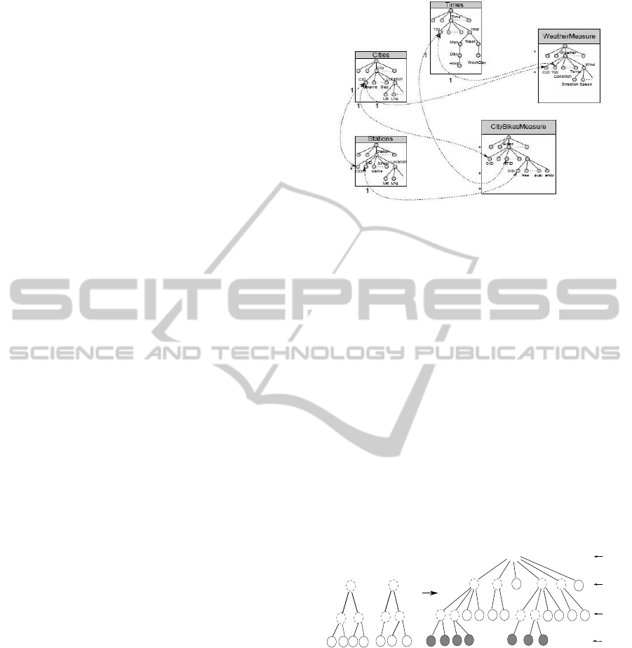
2.2 XML Data Cube Construction

The Data Warehouse (DW) deﬁnition is different

from the schema of the underlying native XML

database. The DW deﬁnition includes a high level de-

scription of all the dimensions and the fact data and

the relationships between them (as shown in Fig.1).

In contrast, the schema of the XML database focuses

on the low-level logical and physical structure of the

XML data. The initial web generated raw sensor data

must be transformed and mapped to the structure de-

scribed by our DW deﬁnition illustrated in Fig.1 It is

not necessary to permanently materialize the identi-

ﬁer information in order to build up the XML DW

Figure 1: An example of logical model for the data ware-

house in CityBikes Project (Gui and Roantree, 2013).

galaxy model and to specify the relationships between

the different parts. (Gui and Roantree, 2013) The

cube deﬁnition details the key components of the cube

construction process: selected dimensions, selected

concept hierarchy within dimensions, measurements

of fact data and aggregating functions. This informa-

tion can be used to determine both the construction

process and the production of the data cube. In our

project, we have developed several XML Schemata

to model the data cube structure, which we name the

XML Data Cube Model (XDCM). The data cube can

be serialized into XML data and an associated index

may be generated to facilitate OLAP operations on

the data cube. Both the serialized XML data cube

and the corresponding index (not discussed in this pa-

per) may be stored into the underlying native XML

database and be made available to related data analy-

sis applications.

p1 p2

all

p1 p2

...

0-D

1-D

2-D

3-D

s1 s2

Figure 2: XDCM cube tree construction demonstration.

In Fig.2, the forest on the left side is a simple illus-

tration of the input XML data concerning bikes usage,

which contains source information to be aggregated.

To simplify the example, we only selected three di-

mensions and each dimension has no more than two

different values. In the input forest, every node at each

level may be repeated an arbitrary number of times.

In the CityBike project, the system generates the data

regularly, and in some dimensions, the domains are

quite limited regarding the number of stations and the

weather details. This will result in a large quantity

of mergers in subsequent operations. The height of

WEBIST2014-InternationalConferenceonWebInformationSystemsandTechnologies

194

input tree is equivalent to the dimension in the DW.

Assuming the dimension of input data is D, then we

will get 2

views to observe the data, including di-

mension 0 . Our XDCM must be robust enough to

describe all the views directly without any join or re-

lated operations. In the case of the forest on the left

side in Fig.2, using the capital letters to represent the

dimensions, we could get C − S − P, C − P, C − S,

S− P,C, S, P and Φ. In fact, C− S−P includesC− S

and C, S − P includes S. From a tree’s point of view,

you must visit the nodes from top to bottom along the

paths. If you have reached P, it follows that you have

already reached C and S. To reduce the redundancy,

some views that are included by others will not be

generated directly in the XDCM. In other words, all

the branches of XDCM cube tree should end with the

nodes in P in this demonstration. The Φ view is the

“all” in the XDCM cube tree at level 0.

The tree on the right side is the XDCM tree be be

constructed. There are three kinds of nodes that will

be used to ﬁnalise the construction.

• Data Node. The gray nodes in Fig.2 represent

the Data Nodes. After several processes such as

ﬁltration or combination (if required), the initial

data can be generated on the Data Nodes directly.

The Data Nodes contain basic information such as

paths and values, and they describe the view with

the longest path such as C − S − P highlighted in

the previous example.

• Additional Node. The Additional Node (indi-

cated by a dashed-circle in Fig.2) which is pro-

duced by the Data Node is a form of intermedi-

ate data not shown in Fig.2. Each Data Node will

produceall possibleAdditional Nodes through the

removal of any constraints in the different dimen-

sions in its path.

• Link Node. The white nodes represent the Link

Nodes which describe other additions paths of ob-

servation. Link Nodes are produced by combin-

ing Additional Nodes that share the same paths.

Nodes in different paths should be unique in the

XDCM.

During the cube construction, for example, Data

Node all − c1 − s1 − p1 will produce Additional

Nodes all − c1 − p1, all − s1 − p1, all − p1, and

Data Node all − c1 − s2 − p1 will produce Addi-

tional Nodes all − c1 − p1, all − s2 − p1, all − p1.

Thus, there are two pairs of nodes that share the same

paths. They are all − s1 − p1 and all − p1. Upon

combination of these nodes, we obtain Link Nodes

all−c1− p1, all−s1− p1, all−s2− p1 and all− p1.

Both Data Nodes and Link Nodes are the nodes in P.

Other nodes describe other views can be calculated in

following processes.

2.3 Map-Reduce

MapReduce is a programming framework for pro-

cessing large data sets with a parallel, distributed al-

gorithm on clusters. The most important functions

in this model are Map and Reduce. Mappers receive

a collection of Key-Value pairs and produce zero or

more output Key-Value pairs. Pairs sharing the same

key are collected and delivered to the same Reducer.

Reducers can iterate through the values that are asso-

ciated with that keyand produce zero or more outputs.

Hadoop has implemented this programming model

and offers a well-deﬁned set of APIs to control the

entire process.

In Hadoop, a complete Map-Reduce task can be

regarded as a job. To ﬁnish an entire task, it may be

necessary to perform more than one job. Input data is

split into many parts and transformed into Key-Value

pairs. In this context, the concept of split is about

a logical rather than a physical operation. Conse-

quently, the data uploaded to the Hadoop Distributed

File System (HDFS) will be cut into several blocks,

usually in 64MB chunks, according to the require-

ments of the system. Hadoop is quite adept at deal-

ing with unstructured data, such as text, because it is

easy to split and suitable for the physical structure.

Hadoop does not offer any functionality to process

XML documents directly. Mahout, an open-source

program based on Hadoop, provides a class to handle

the XML input format, and the underlying strategy

is simple. An XML document is well organized, the

content of every element is enclosed by a pair of tags.

Therefore, it is sufﬁcient to simply read the XML doc-

ument as a text ﬁle and select the content between the

certain pair of tags.

3 CUBE CONSTRUCTION WITH

MAP-REDUCE

In order to describe the algorithm, consider an exer-

cise to build an OLAP data cube for the bicycle rental

scenario under certain weather conditions and in var-

ious locations and dates. In this case, only three di-

mensions have been chosen as shown in Fig.2. The

Input data are nodes in the dimension named P with

some additional information, such as their path con-

straints. On the left side, the nodes indicated with a

dashed-circle illustrate the paths of the nodes circled

by solid lines, and they do not need to be instantiated.

Our goal is to build the tree on the right side and to

calculate the values of the dashed nodes.

DataCubeComputationalModelwithHadoopMapReduce

195

For our implementation, the entire task can be di-

vided into two phases. Phase one is to generate the

Data Nodes and Link Nodes, and then organize them

into the XDCM as described earlier. The second

phase is to calculate the values of the dashed nodes

on the right side which represent observation views

other than Data Nodes and Link Nodes. The calcu-

lation task itself can be divided into two further sub-

tasks. One subtask is used for the calculation of Data

Nodes and the other subtask is used for the calculation

of Link Nodes.

all

......

leaf1 leaf2 leaf3 leaf4 ······

b3 b4

n-1

Figure 3: Processing Order of Data Nodes.

all

Figure 4: Processing Order of Link Nodes.

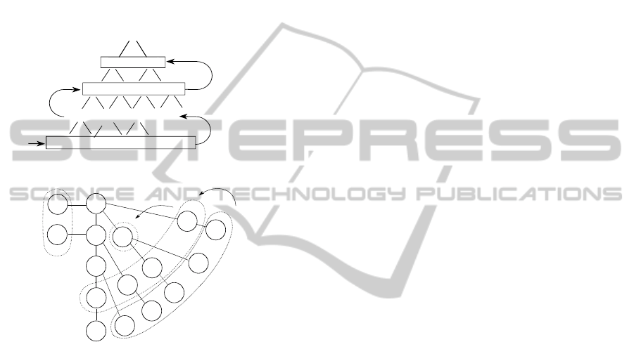
Fig.3 illustrates the node processing order of the

algorithm. The integer values on the right side rep-

resent the round indexes of Map-Reduce jobs. Data

Nodes are the leaf nodes shown at the bottom, and

they will be processed by the ﬁrst job to generate Ad-

ditional Nodes. The Additional Nodes will subse-

quently be merged into Link Nodes. Thus, the sub-

sequent rounds only concentrate on the calculation

tasks. For a N-dimensional XML data, we need at

least N rounds to complete the entire construction,

in other words, N jobs are needed to complete the

whole task in Hadoop. The output generated from

each job will be used as the input data for the next job.

The computation receives a set of Key-Value pairs as

input, and then produces a set of output Key-Value

pairs:

Map (k1, v1) → list(k2, v2)

Reduce (k2, list(v2)) → (k3, v3)

In the generation phase (phase one), the initial

data is transformed into Key-Value pairs that actu-

ally represent Data Nodes. So k1 is the path of a

given Data Node, and v1 is the value of that node.

Data Nodes will produce large amounts of Additional

Nodes. k2 is the path of an Additional Node, and v2 is

its value. The Reduce function accepts the intermedi-

ate key k2 and a set of values for that key, and merges

these values to form a Link Node. So k3 is the path of

Link Node, and v3 is the actual value.

In the calculation phase (phase two), the process

starts with either the Data Nodes or the Link Nodes.

All nodes in the same level will be processed in one

job. The entire process proceeds in a bottom-up man-

ner from one layer to the next. However, unlike the

generation phase, the Key value of the Mapper’s out-

put is the path of the node without self-containment.

For example, given the input node γ and the path

α − β − γ. Then k2 will be α − β , and v2 will be

γ. The Reduce function accepts the intermediate key

α − β and calculates the value of β. The k3 is the

complete path of β which is α − β, and v3 is β. This

(k3, v3) pair will be the (k1, v1) in the next calculation

round, which is going to calculate the value of α.

Given that all Link Nodes are derived from Data

Nodes and all nodes in the XDCM are unique, some

ancestor nodes may be calculated using different de-

scendants in different paths. For example, in Fig.4,

the node B in all − B − C − D may be calculated by

all − B− D also. To avoid repeated calculations, we

employ a ”BreakPoint” to indicate the point at which

to stop the calculation. The procedure for selecting a

BreakPoint in the basic implementation is as follows:

1. The BreakPoint represents a node in a path. If the

BreakPoint is going to be calculated in the next

round, the calculation should be stopped.

2. Only Link Nodes and their ancestor nodes need

to keep a record of BreakPoints. All nodes in the

path of Data Nodes will be calculated. So it is un-

necessary to keep records of BreakPoints for Data

Nodes and their ancestor nodes.

3. BreakPoints are identiﬁed in the generation phase

and won’t change in the following calculations.

The ancestor nodes of each Link Node should in-

herit its BreakPoint.

4. It should be noted that BreakPoints are the places

where new branches are added while building the

XDCM cube tree. For instance, in Fig.4, all the

branches except all − A− B−C− D are branches

that were added. As for all − A − C − D, the

BreakPoints are the nodes at A, because −C− D

is the branch we added.

Fig.4 shows the abstract structure of XDCM in

four dimensions. As described in section 2.2, the

paths of all nodes start from all and end at D. Thus,

the total number of Link Nodes is the combinations

WEBIST2014-InternationalConferenceonWebInformationSystemsandTechnologies

196

from A to C minus one (because we already have the

longest path, A−B−C). For the N-dimensional data,

the number of Additional Nodes for each Data Node

is C

N−2

N−1

N−3

N−1

+ ... +C

N−1

(N ≥ 2).

In our implementation, we use binary numbers to

describe the status of those combinations. In Fig.4,

the number of Additional Nodes for each Data Node

is C

= 7. So using three bits (2

(3−1)

) can

describe all cases. Each bit stands for a dimension

between all to D. If a certain bit is set to 1, it indicates

having the constraint on that dimension. To identify

a BreakPoint for each Link Node, we need to check

whether the preﬁx of the Link Node’s path has already

existed in the tree that we have currently built. we

may enumerate all of the cases by reducing the binary

number from the maximum to zero. We determine the

BreakPoint by comparing the preﬁx of two adjacent

cases. The maximum of the binary number should

compare with the binary number that stands for the

Data Node. In the previous example, the 110 should

compare with 111, so the BreakPoint for 110 is at the

second bit which represents the B dimension. If there

is no common substring in the preﬁx (as with 100 and

011), the BreakPoint for 011 is the node all.

4 OPTIMIZATION AND

PERFORMANCE

4.1 Conﬁguration Optimization

We performed the experiments in a cluster with 35

slave nodes each containing a 3.10GHz processor, 1

GB of RAM, and 40 GB of local disk allocated to the

HDFS. Each node is running Hadoop version 1.1.2

on Red Hat 9.0 and connected by Fast Ethernet to a

commodity router.

An XML document contains more information

than an unstructured document with equivalent con-

tent. In order to handle XML documents in a dis-

tributed system without loss of information we need

to restructure the data and divide it into small units.

Thus, the amount of data through the system is larger

than the input data. The table in Fig.5 shows the size

of the data and the number of records through the sys-

tem in the ﬁrst round.

Each record in Hadoop represents a unit we made

which is described as a node in section two and

Dimension Map input

bytes

Map

output

bytes

Map output

records

Reduce input

records

Reduce input

records(after

combining)

1,023,266,669

4,973,220,180

126,360,000

35,101,440

5,386,519,202

24,703,200,180

622,080,000

180,001,136

1,104,659,389

44,683,382,133

1,075,164,192

51,916,510

5,514,648,663

130,268,589,390

2,686,965,696

250,036,747

Figure 5: comparing the data through the system in the ﬁrst

round.

three. In the experiments, we use two types of XML

ﬁles for the experiments, of three-dimensions and six-

dimension respectively. The arity of each dimension

is nine. For 1 GB XML ﬁle in three dimensions, us-

ing the basic algorithm, the Map output in the ﬁrst job

is about 4.6 GB. In other words, to build the XDCM

directly, the size of data we actually need is approxi-

mately 4.6 GB. For 1 GB XML ﬁle in six dimensions,

using the basic algorithm, the Map output in the ﬁrst

job reaches 41 GB. Since Mappers and Reducers are

separated, these outputs are transferred through the

network. The I/O operations may have a negative im-

pact on the whole task.

Hadoop offers several ways to optimize the I/O.

In the experiments, we mainly used compression and

combination, and their effects were clear. Hadoop

supports several compression formats like gzip and

snappy. The compression method should be selected

according to the type of the task to be performed. If

the task’s CPU occupancy rate is high, it is better to

choose a simple compression algorithm. If a signiﬁ-

cant portion of the task is spent at I/O, it is better to

select an algorithm with a high compression ratio. in

our experiment, using the default compression algo-

rithm offered by Hadoop to process 1 GB of XML

data in three dimensions provides approximately an

8% improvement.

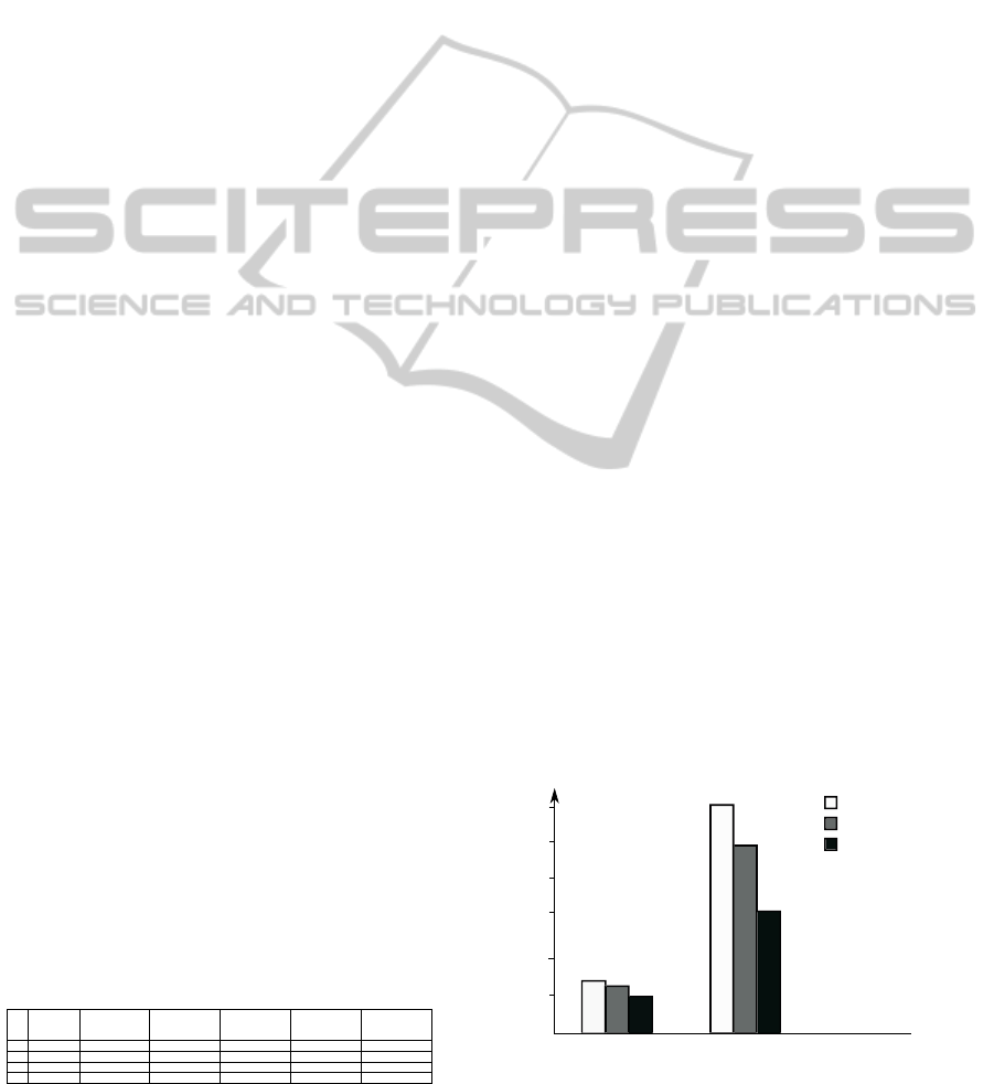
In our experiments, the combination process pro-

vided a demonstrable improvement. The task of a

Combiner is similar to that of a Reducer. If the Com-

biner is used then the outputs from the Mapper are

not immediately delivered to the Reducer. The Key-

Value pairs are collected in lists, one list per Key. The

Combiner will process each list like a Reducer and

emit a new Key-Value pair which has already been

merged. Then the new Key-Value pair will be deliv-

ered to the Reducer as if they were created by the orig-

inal Map operation. Fig.6 shows the performance us-

ing these two strategies when dealing with the three-

dimensional XML ﬁles.

21'12"

17'36''

12'1''

4'36''

4'12''

2'48''

compress

compress&&combine

original

1 GB XML 5 GB XML

minute

Figure 6: Performance of Optimization for 3-D XML.

DataCubeComputationalModelwithHadoopMapReduce

197

4.2 Algorithm Optimization

For the 1 GB and three-dimensional XML ﬁle in

our experiment, using the basic algorithm discussed

in section 3, the number of Map output records is

about 126,360,000in the ﬁrst round but the number of

Reduce output records is approximately 35,101,440.

About 72% records are merged in Reducers. For the

1 GB and six-dimensional XML ﬁle, the number of

Map output records is approximately 1,075,164,192

but the number of Reduce output records is only

51,9156,510. The gap in the 5 GB ﬁle sizes is even

more pronounced. As the dimension increases, the

output of Map increases more rapidly. For a D-

dimensional XML ﬁle, assuming n is the number of

initial Data Nodes, the direct output records of Map

is 2

× n . In the basic algorithm, the workload is too

large when the dimension becomes higher in the ﬁrst

round. Too much data is transferred from the Mapper

to the Reducer. In a cloud environment with limited

capacity, it may increase the risk of the jobs failing.

In the basic algorithm, all Additional Nodes come

from Data Nodes. However, some nodes can be gen-

erated by Link Nodes also. The Link Nodes with

longer paths can produce the Additional Nodes with

shorter paths. In Fig.4, Nodes in all − D can not only

be generated by all − A − B − C − D (Data Nodes),

but also can be generated by other six types of Link

Nodes like all−A−B−D, all−B−D, etc. Although

the information in all − A − B − D or all − B − D is

not as complete as the Data Nodes, it is enough for

all − D. The signiﬁcant advantage of using shorter-

path nodes to generate Link Nodes is the decrease in

the I/O between Mapper and Reducer. For example,

there are only two Data Nodes, the paths of which are

all − a1− b1− c1 − d1 and all − a2 − b1 − c1− d1.

Thus, the Link Node in all − B−D will be all −b1−

d1. It is more efﬁcient to generate the Link Node in

all − D by using Link Node all − b1− d1 instead of

using the Data Nodes because only one output record

is produced by the Mapper, whereas the Data Nodes

would produce two.

Fig.7 is an example of generating Link Nodes

by using an optimized algorithm for ﬁve-dimensional

data. As discussed in section 3, all of the pos-

sible Link Nodes for ﬁve-dimensional Data Nodes

(all − A − B − C − D − E) depend on combinations

of the path between all and E exclusively, which is

A − B − C − D. In the ﬁrst round, by removing one

constraint in the path A− B−C− D, we get C

kinds

of Link Nodes shown in column 1 in Fig.7. The arrow

above the node is the indicator of a BreakPoint. The

arrow pointing to empty means the BreakPoint is at

all. Any Link Node whose BreakPoint does not point

A B C

A B D

A C D

B C D

B C

A B

B D

C D

2 1 3

Figure 7: Using Link Nodes for Generation.

to all can be used to generate new Link Nodes in the

next round. In the next round, another constraint of

the Link Nodes is to be removed, and this constraint

should be the nodes before the BreakPoint. As shown

in Fig.7, the A−B−C in column 1 stands for the Link

Nodes whose path is all − A− B−C− E. The Break-

Point is at C, so in next round shown in column 2,

successively removing the nodes before C (including

C), which are C, B, A, we obtain A− B, A−C, B−C.

The BreakPoint changes to the point at the node be-

fore the node has been removed. If the BreakPoint

points at all like B−C, it would not participate in the

generation work of future rounds, but the calculation

phase would continue. In this way, we obtain all of

the combinations after the removal of two constraints

from the path, which is C

in total. The Link Nodes

are generated according to the rules described above,

until all BreakPoints point to all. The total number is

+ C

= 15, which is the same number

produced by the basic algorithm.

Assuming the dimension is D, in the Nth round,

the number of Additional nodes for each Link Node

is C

D−1

. It would appear that the I/O should increase

when N is close to

D−1

. However, it does not because

the Additional Nodes are produced by Link Nodes in-

stead of Data Nodes, and after several rounds of merg-

ers, the number of Link Nodes decrease signiﬁcantly.

The total outputs from the Mapper after N rounds are

still less than the ﬁrst round in our experiment.

Fig.8 shows the different efﬁciencies obtained

by employing these two algorithms to construct the

XDCM using the six-dimensional XML data. The

improvement in the performance is signiﬁcant. For

the 1 GB and 6-dimensional XML ﬁle, the total im-

provement is approximately 64%. For the 5 GB and

6-dimensional XML ﬁle, the improvement is approx-

imately 27%. Fig.9 shows the the performance of the

two algorithms using the 5GB XML data from City-

Bikes.

WEBIST2014-InternationalConferenceonWebInformationSystemsandTechnologies

198

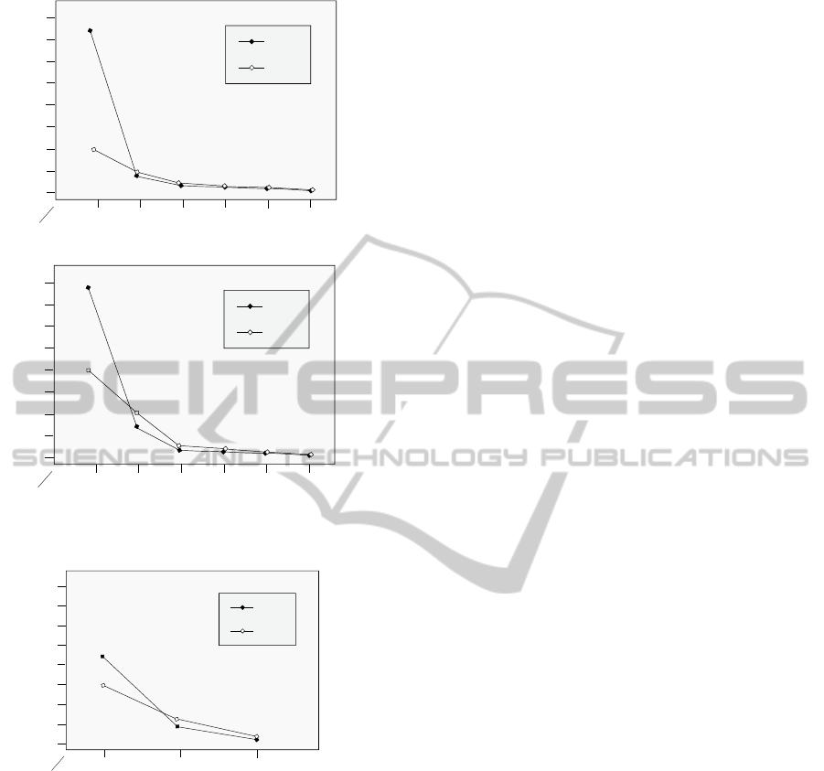
basic

optimized

min

round

1 GB XML in 6 dimensions

basic

optimized

min

round

5 GB XML in 6 dimensions

Figure 8: Basic Algorithm vs. Optimized Algorithm.

basic

optimized

min

round

Figure 9: Performance in CityBike.

5 CONCLUSIONS

In this paper, we illustrated a data cube model for

XML documents to meet the increasing demand for

analyzing massive XML data in OLAP. Hadoop is a

popular framework aiming at tackling large-scale data

problems. We proposed a basic algorithm to construct

the XDCM on Hadoop. To improve efﬁciency, we of-

fered some strategies and described an optimized al-

gorithm. The result proves the optimized algorithm is

suitable for this type of data and further enhance the

efﬁciency.

REFERENCES

Dede, E., Fadika, Z., Gupta, C., and Govindaraju, M.

(2011). Scalable and distributed processing of scien-

tiﬁc xml data. In Proceedings of the 2011 IEEE/ACM

12th International Conference on Grid Computing,

pages 121–128. IEEE Computer Society.

Dutta, H., Kamil, A., Pooleery, M., Sethumadhavan, S.,

and Demme, J. (2011). Distributed storage of large-

scale multidimensional electroencephalogram data us-

ing hadoop and hbase. In Grid and Cloud Database

Management, pages 331–347. Springer.

Gui, H. and Roantree, M. (2012). A data cube model for

analysis of high volumes of ambient data. Procedia

Computer Science, 10:94–101.

Gui, H. and Roantree, M. (2013). Using a pipeline approach

to build data cube for large xml data streams. In

Database Systems for Advanced Applications, pages

59–73. Springer.

Khatchadourian, S., Consens, M. P., and Sim´eon, J. (2011).

Having a chuql at xml on the cloud. In AMW.

Lin, J. and Schatz, M. (2010). Design patterns for efﬁ-

cient graph algorithms in mapreduce. In Proceedings

of the Eighth Workshop on Mining and Learning with

Graphs, pages 78–85. ACM.

Rusu, L. I., Rahayu, W., and Taniar, D. (2009). Partition-

ing methods for multi-version xml data warehouses.

Distributed and Parallel Databases, 25(1-2):47–69.

DataCubeComputationalModelwithHadoopMapReduce

199