Exploiting Local Class Information in Extreme Learning Machine
Alexandros Iosifidis, Anastasios Tefas and Ioannis Pitas
Department of Informatics, Aristotle University of Thessaloniki, Thessaloniki, Greece
Keywords:
Single-hidden Layer Feedforward Neural Networks, Extreme Learning Machine, Facial Image Analysis.
Abstract:
In this paper we propose an algorithm for Single-hidden Layer Feedforward Neural networks training. Based
on the observation that the learning process of such networks can be considered to be a non-linear mapping
of the training data to a high-dimensional feature space, followed by a data projection process to a low-
dimensional space where classification is performed by a linear classifier, we extend the Extreme Learning
Machine (ELM) algorithm in order to exploit the local class information in its optimization process. The
proposed Local Class Variance Extreme Learning Machine classifier is evaluated in facial image classification
problems, where we compare its performance with that of other ELM-based classifiers. Experimental results
show that the incorporation of local class information in the ELM optimization process enhances classification
performance.
1 INTRODUCTION
Extreme Learning Machine is a relatively new algo-
rithm for Single-hidden Layer Feedforward Neural
(SLFN) networks training (Huang et al., 2004) that
leads to fast network training requiring low human su-
pervision. Conventional SLFN network training algo-
rithms require the input weights and the hidden layer
biases to be adjusted using a parameter optimization
approach, like gradient descend. However, gradient
descend-based learning techniques are generally slow
and may decrease the network’s generalization abil-
ity, since they may lead to local minima. Unlike the
popular thinking that the network’s parameters need
to be tuned, in ELM the input weights and the hidden
layer biases are randomly assigned. The network out-
put weights are, subsequently, analytically calculated.
ELM not only tends to reach the smallest training er-
ror, but also the smallest norm of output weights. As
shown in (Bartlett, 1998), for feedforward networks
reaching a small training error, the smaller the norm
of weights is, the better generalization performance
the networks tend to have. Despite the fact that the
determination of the network hidden layer output is
a result of randomly assigned weights, it has been
shown that SLFN networks trained by using the ELM
algorithm have the properties of global approxima-
tors (Huang et al., 2006). Due to its effectiveness and
its fast learning process, the ELM network has been
widely adopted in many classification problems, in-
cluding facial image classification (Zong and Huang,
2011; Rong et al., 2008; Lan et al., 2008; Helmy and
Rasheed, 2009; Huang et al., 2012; Iosifidis et al.,
2013d; Iosifidis et al., 2013b; Iosifidis et al., 2013a;
Iosifidis et al., 2014a; Iosifidis et al., 2014c).
Despite its success in many classification prob-
lems, the ability of the original ELM algorithm to
calculate the output weights is limited due to the fact
that the network hidden layer output matrix is, usu-
ally, singular. In order to address this issue, the Ef-
fective ELM (EELM) algorithm has been proposed
in (Wang et al., 2011), where the strictly diago-
nally dominant criterion for nonsingular matrices is
exploited, in order to choose proper network input
weights and bias values. However, the EELM al-
gorithm has been designed only for a special case
of SLFN networks employing Gaussian Radial Ba-
sis Functions (RBF) for the input layer neurons. In
(Huang et al., 2012), an optimization-based regular-
ized version of the ELM algorithm (ORELM) aiming
at both overcoming the full rank assumption for the
network hidden layer output matrix and at enhancing
the generalization properties of the ELM algorithm
has been proposed. ORELM has been evaluated on
a large number of classification problems providing
very satisfactory classification performance.
By using a sufficiently large number of hidden
layer neurons, the ELM classification scheme, when
approached from a Discriminant Learning point of
view (Iosifidis et al., 2013c), can be considered as a
49
Iosifidis A., Tefas A. and Pitas I..
Exploiting Local Class Information in Extreme Learning Machine.
DOI: 10.5220/0005038500490055
In Proceedings of the International Conference on Neural Computation Theory and Applications (NCTA-2014), pages 49-55
ISBN: 978-989-758-054-3
Copyright
c
 2014 SCITEPRESS (Science and Technology Publications, Lda.)

learning process formed by two processing steps. The
first step corresponds to a mapping process of the in-
put space to a high-dimensionalfeature space preserv-
ing some properties of interest for the training data.
In the second step, an optimization scheme is em-
ployed for the determination of a linear projection of
the high-dimensional data to a low-dimensional fea-
ture space determined by the network target vectors,
where classification is performed by a linear classifier.
Based on this observation, the ORELM algorithm has
been extended in order to exploit discriminative crite-
ria in its optimization process (Iosifidis et al., 2013c).
Specifically, it has been shown that the incorporation
of the within-class scatter in the optimization process
followed for the calculation of the network output
weights enhanced the ELM network performance.
In this paper, we follow this line of work and
propose an extension of the ELM algorithm which
exploits local class information in the optimization
problem solved for the determination of the network
output weights, in order to further increase the ELM
network performance. The proposed Local Class
Variance ELM (LCVELM) algorithm aims at mini-
mizing both the network output weights norm and the
within class variance of the training data in the ELM
space, expressed by employing locality constraints.
We evaluate the proposed LCVELM network in fa-
cial image classification problems, where we compare
its performance with that of the ELM (Huang et al.,
2004), ORELM (Huang et al., 2012) and MCVELM
(Iosifidis et al., 2013c) networks. Experimental re-
sults denote that the incorporation of local class in-
formation in the ELM optimization problem enhances
facial image classification performance.
The paper is structured as follows. In Section 2 we
briefly describe the ELM algorithm. In Section 3, we
describe the proposed LCVELM algorithm for SLFN
network training. Section 4 presents experiments con-
ducted in order to evaluate its performance. Finally,
conclusions are drawn in Section 5.
2 THE ELM ALGORITHM
The ELM network has been proposed for supervised
classification (Huang et al., 2004). Let us denote by
{x
i
, c
i
}, i = 1, . . . , N a set of N vectors x
i
∈ R
D
fol-
lowed by class labels c
i
∈ {1, . . . ,C} . We would like
to employ them in order to train a SLFN network.
Such a network consists of D input (equal to the di-
mensionality of x
i
), L hidden and C output (equal to
the number of classes involved in the classification
problem) neurons. The number of hidden layer neu-
rons is usually selected to be much greater than the
number of classes (Huang et al., 2012; Iosifidis et al.,
2013c), i.e., L ≫ C.
The network target vectors t
i
= [t
i1
, ...,t
iC
]
T
, each
corresponding to a training vector x
i
, are set to t
ik
= 1
for vectors belonging to class k, i.e., when c
i
= k, and
to t
ik
= −1 otherwise. The network input weights
W
in
∈ R
D×L
and the hidden layer bias values b ∈
R
L
are randomly assigned, while the network output
weights W
out
∈ R
L×C
are analytically calculated. Let
us denote by v
j
the j-th column of W
in
, by w
k
the k-th
row of W
out
and by w
kj
the j-th element of w
k
. For a
given activation function for the network hidden layer
Φ(·) and by using a linear activation function for the
network output layer, the output o
i
= [o
1
, . . . , o
C
]
T
of
the network corresponding to x
i
is calculated by:
o
ik
=
L
∑
j=1
w
kj
Φ(v
j
, b
j
, x
i
), k = 1, ...,C. (1)
It has been shown (Huang et al., 2012) that, sev-
eral activation functions Φ(·) can be used for the cal-
culation of the network hidden layer outputs, like the
sigmoid, sine, Gaussian, hard-limiting and Radial Ba-
sis Functions (RBF). The most widely adopted choice
is the sigmoid function, defined by:
Φ(v
j
, b
j
, s
i
) =
1
1+ e
−(v
T
j
s
i
+b
j
)
. (2)
By storing the network hidden layer outputs cor-
responding to the training vectors x
i
, i = 1, . . . , N in a
matrix Φ:
Φ =



Φ(v
1
, b
1
, x
1
) ··· Φ(v
1
, b
1
, x
N
)
···
.
.
.
···
Φ(v
L
, b
L
, x
1
) ··· Φ(v
L
, b
L
, x
N
)



, (3)
equation (1) can be expressed in a matrix form as:
O = W
T
out
Φ. (4)
Finally, by assuming that the predicted network out-
puts O are equal to the network targets, i.e., o
i
=
t
i
, i = 1, ..., N, W
out
can be analytically calculated by:
W
out
= Φ
†
T
T
, (5)
where Φ
†
=

ΦΦ
T

−1
Φ is the Moore-Penrose gener-
alized pseudo-inverse of Φ
T
and T = [t
1
, . . . , t
N
] is a
matrix containing the network target vectors.
The ELM algorithm assumes zero training error.
However, in cases where the training data contain out-
liers, this assumption may reduce its potential in gen-
eralization. In addition, since the dimensionality of
the ELM space is usually high, i.e., in some cases
L > N, the matrix B = ΦΦ
T
is singular and, thus,
the adoption of (5) for the calculation of the network
output weights is inappropriate. By allowing small
NCTA2014-InternationalConferenceonNeuralComputationTheoryandApplications
50

training errors and trying to minimize the norm of the
network output weights, W
out
can be calculated by
minimizing (Huang et al., 2012):
J
ORELM
=
1
2
kW
out
k
2
F
+
c
2
N
∑
i=1
kξ
i
k
2
2
, (6)
W
T
out
φ
i
= t
i
− ξ
i
, i = 1, ..., N, (7)
where ξ
i
∈ R
C
is the error vector corresponding to x
i
and c is a parameter denoting the importance of the
training error in the optimization problem. φ
i
is the
i-th column of Φ, i.e., the hidden layer output corre-
sponding x
i
. That is, φ
i
is the representation of x
i
in
R
L
. By substituting (7) in J
ORELM
(6) and determin-
ing the saddle point of J
ORELM
, W
out
is given by:
W
out
=

ΦΦ
T
+
1
c
I

−1
ΦT
T
. (8)
The adoption of (12) for W
out
calculation, instead
of (5), has the advantage that the matrix B =

ΦΦ
T
+
1
c
I

is nonsingular, for c > 0.
By allowing small training errors and trying
to minimize both the norm of the network output
weights and the within-class variance of the training
vectors in the projection space, W
out
can be calcu-
lated by minimizing (Iosifidis et al., 2013c):
J
MCVELM
= kS
1
2
w
W
out
k
2
F
+ λ
N
∑
i=1
kξ
i
k
2
2
, (9)
W
T
out
φ
i
= t
i
− ξ
i
, i = 1, ..., N, (10)
where S
w
is the within-class scatter matrix used in
Linear Discriminant Analysis (LDA) (Duda et al.,
2000) describing the variance of the training classes
in the ELM space and is defined by:
S
w
=
C
∑
j=1
∑
i,c
i
= j
1
N
j
(φ
i
− µ
j
)(φ
i
− µ
j
)
T
. (11)
In (11), N
j
is the number of training vectors belonging
to class j and µ
j
=
1
N
j
∑
i,c
i
= j
φ
i
is the mean vector of
class j. By calculating the within-class scatter matrix
in the ELM space R
L
, rather than in the input space
R
D
, nonlinear relationships between training vectors
forming the various classes can be better described.
By substituting (10) in J
MCVELM
and determining the
saddle point of J
MCVELM
, W
out
is given by:
W
out
=

ΦΦ
T
+
1
c
S
w

−1
ΦT
T
. (12)
Since the matrix B =

ΦΦ
T
+
1
c
S
w

is not always
nonsingular, an additional dimensionality reduction
processing step perfomred by applying Principal
Component Analysis (Duda et al., 2000) on Φ has
been proposed in (Iosifidis et al., 2013c). Another
variant that exploits the total scatter matrix of the en-
tire training set has been proposed in (Iosifidis et al.,
2014b).
3 THE LCVELM ALGORITHM
In this Section, we describe the proposed Local Class
Variance LM (LCVELM) algorithm for SLFN net-
work training. Similar to the ELM variance described
in Section 2, the proposed algorithm exploits ran-
domly assigned network input weights W
in
and bias
values b, in order to perform a nonlinear mapping of
the data in the (usually high-dimensional) ELM space
R
L
. After the network hidden layer outputs calcula-
tion, we assume that the data representations in the
ELM space φ
i
, i = 1, . . . , N are embedded in a graph
G = {V , E, W}, where V denotes the graph vertex
set, i.e., V = { φ
i
}
N
i=1
, E is the set of edges connecting
φ
i
, and W ∈ R
N×N
is the matrix containing the weight
values of the edge connections. Let us define a simi-
larity measure s(·, ·) that will be used in order to mea-
sure the similarity between two vectors (Yan et al.,
2007). That is, s
ij
= s(φ
i
, φ
j
) is a value denoting the
similarity between φ
i
and φ
j
. s(·, ·) may be any simi-
larity measure providing non-negativevalues (usually
0 ≤ s
ij
≤ 1). The most widely adopted choice is the
heat kernel (also known as diffusion kernel) (Kondor
and Lafferty, 2002), defined by:
s(φ
i
, φ
j
) = exp
−
kφ
i
−φ
j
k
2
2
2σ
2
, (13)
where k · k
2
denotes the l
2
norm of a vector and σ
is a parameter used in order to scale the Euclidean
distance between φ
i
and φ
j
.
In order to express the local intra-class relation-
ships of the training data in the ELM space, we ex-
ploit the following two choices for the determination
of the weight matrix W:
W
(1)
ij
=

1 if c
i
= c
j
and j ∈ N
i
,
0, otherwise,
or
W
(2)
ij
=

s
ij
if c
i
= c
j
and j ∈ N
i
,
0, otherwise.
In the above, N
i
denotes the neighborhood of φ
i
(we
have employed 5-NN graphs in all our experiments).
W
(1)
has been successfully exploited for discriminant
subspace learning in Marginal Discriminant Analysis
(MDA) (Yan et al., 2007), while W
(2)
can be consid-
ered to be modification of W
(1)
, exploiting geomet-
rical information of the class data. A similar weight
ExploitingLocalClassInformationinExtremeLearningMachine
51

matrix has also been exploited in Local Fisher Dis-
criminant Analysis (LFDA) (Sugiyama, 2007). In
both MDA and LFDA cases, it has been shown that by
exploiting local class information enhanced class dis-
crimination can be achieved, when compared to the
standard LDA approach exploiting global class infor-
mation, by using (11).
After the calculation of the graph weight matrix
W, the graph Laplacian matrix L
N×N
is given by
(Belkin et al., 2007):
L = D− W, (14)
where D is a diagonal matrix with elements D
ii
=
∑
N
j=1
W
ij
.
By exploiting L, the network output weights W
out
of the LCVELM network can be calculated by mini-
mizing:
J
LCVELM
=
1
2
kW
out
k
2
F
+
c
2
N
∑
i=1
kξ
i
k
2
2
+
λ
2
tr

W
T
(ΦLΦ
T
)W

, (15)
W
T
out
φ
i
= t
i
− ξ
i
, i = 1, ..., N, (16)
where tr(·) is the trace operator. By substituting the
constraints (16) in J
LCVELM
and determining the sad-
dle point of J
LCVELM
, the network output weights
W
out
are given by:
W
out
= Φ

I+
λ
c
L

Φ
T
+
1
c
I
!
−1
ΦT
T
. (17)
Similar to (12), the calculation of the network output
weights by employing (17) has the advantage that the
matrix B = Φ

I+
λ
c
L

Φ
T
+
1
c
I
!
is nonsingular,
for c > 0. In addition, the calculation of the graph
similarity values s(·, ·) in the ELM space R
L
, rather
than the input space R
D
has the advantage that nonlin-
ear relationships between the training vectors forming
the various classes can be better expressed.
After the determination of the network output
weights W
out
, a test vector x
t
can be introduced to
the trained network and be classified to the class cor-
responding to the maximal network output:
c
t
= argmax
k
o
tk
, k = 1, . . . ,C. (18)
4 EXPERIMENTS
In this section, we present experiments conducted in
order to evaluate the performance of the proposed
LCVELM algorithm. We have employed six pub-
licly available datasets to this end. These are: the
ORL, AR and Extended YALE-B (face recognition)
and the COHN-KANADE, BU and JAFFE (facial
expression recognition). A brief description of the
datasets is provided in the following subsections. Ex-
perimental results are provided in subsection 4.3. In
all our experiments we compare the performance of
the proposed LCVELM algorithm with that of ELM
(Huang et al., 2004), ORELM (Huang et al., 2012)
and MCVELM (Iosifidis et al., 2013c) algorithms.
The number of hidden layer neurons has been set
equal to L = 1000 for all the ELM variants, a value
that has been shown to provide satisfactory perfor-
mance in many classification problems (Huang et al.,
2012; Iosifidis et al., 2013c). For fair comparison,
in all the experiments, we make sure that the the
same ELM space is used in all the ELM variants.
That is, we first map the training data in the ELM
space and, subsequently, calculate the network output
weights accordingto each ELM algorithm. Regarding
the optimal values of the regularization parameters
c, λ used in the competing ELM-based classification
schemes, they have been determined by following a
grid search strategy. That is, for each classifier, mul-
tiple experiments have been performed by employing
different parameter values (c = 10
r
, r = −3, . . . , 3 and
λ = 10
p
, p = −3, . . . , 3) and the best performance is
reported.
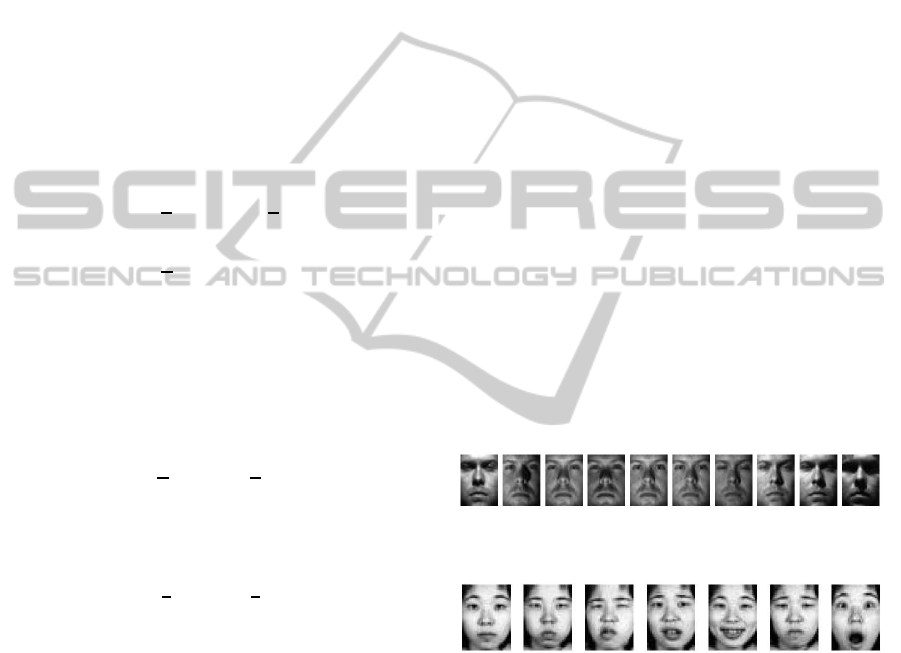
Figure 1: Facial images depicting a person from the Ex-
tended YALE-B dataset.
Figure 2: Facial images depicting a person from the JAFFE
dataset. From left to right: neutral, anger, disgust, fear,
happy, sad and surprise.
4.1 Face Recognition Datasets
4.1.1 The ORL Dataset
It consists of 400 facial images depicting 40 persons
(10 images each) (Samaria and Harter, 1994). The im-
ages were captured at different times and with differ-
ent conditions, in terms of lighting, facial expressions
(smiling/not smiling) and facial details (open/closed
eyes, with/without glasses). Facial images were taken
in frontal position with a tolerance for face rotation
NCTA2014-InternationalConferenceonNeuralComputationTheoryandApplications
52

Table 1: Classification rates on the ORL dataset.
ELM ORELM MCVELM LCVELM (1) LCVELM (2)
10% 30.78% 40.65% 41.01% 41.26% 41.22%
20% 20.67% 39.76% 41.81% 41.81% 41.81%
30% 38.17% 52.11% 55% 55.78% 55.78%
40% 38.31% 53% 57% 57.19% 57.13%
50% 47% 77.62% 75.54% 77.69% 77.77%
Table 2: Classification rates on the AR dataset.
ELM ORELM MCVELM LCVELM (1) LCVELM (2)
10% 66.47% 67.79% 68.87% 69.19% 69.15%
20% 70.49% 80.24% 80.91% 80.86% 80.96%
30% 65.26% 82.98% 81.81% 83.27% 83.1%
40% 75.33% 91.9% 92.94% 93.01% 93.01%
50% 80.33% 94.16% 94.65% 94.9% 94.9%
Table 3: Classification rates on the YALE-B dataset.
ELM ORELM MCVELM LCVELM (1) LCVELM (2)
10% 69.17% 72.22% 72.22% 72.22% 72.22%
20% 83.44% 84.38% 84.38% 85% 84.38%
30% 82.86% 85.36% 85.36% 88.21% 85.36%
40% 90% 92.08% 92.08% 92.5% 92.08%
50% 91% 93.5% 94.5% 94.5% 94.5%
Figure 3: Facial images depicting a person from the ORL
dataset.
and tilting up to 20 degrees. Example images
of the dataset are illustrated in Figure 3.
4.1.2 The AR Dataset
It consists of over 4000 facial images depicting 70
male and 56 female faces (Martinez and Kak, ). In our
experiments we have used the preprocessed (cropped)
facial images provided by the database, depicting 100
persons (50 males and 50 females) having a frontal
facial pose, performing several expressions (anger,
smiling and screaming), in different illumination con-
ditions (left and/or right light) and with some oc-
clusions (sun glasses and scarf). Each person was
recorded in two sessions, separated by two weeks.
Example images of the dataset are illustrated in Fig-
ure 4.
Figure 4: Facial images depicting a person from the AR
dataset.
4.1.3 The Extended YALE-B Dataset
It consists of facial images depicting 38 persons in 9
poses, under 64 illumination conditions (Lee et al.,
2005). In our experiments we have used the frontal
cropped images provided by the database. Example
images of the dataset are illustrated in Figure 1.
4.2 Facial Expression Recognition
Datasets
4.2.1 The COHN-KANADE Dataset
It consists of facial images depicting 210 persons of
age between 18 and 50 (69% female, 31% male, 81%
Euro-American, 13% Afro-American and 6% other
groups) (Kanade et al., 2000). We have randomly
selected 35 images for each facial expression, i.e.,
anger, disgust, fear, happyness, sadness, surprise and
neutral. Example images of the dataset are illustrated
in Figure 5.
Figure 5: Facial images from the COHN-KANADE dataset.
From left to right: neutral, anger, disgust, fear, happy, sad
and surprise.
ExploitingLocalClassInformationinExtremeLearningMachine
53

Table 4: Classification rates on the facial expression recognition dataset.
ELM ORELM MCVELM LCVELM (1) LCVELM (2)
COHN-KANADE 49.8% 79.59% 80% 80.41% 80%
BU 65% 71,57% 71,57% 72% 72,86%
JAFFE 47.62% 58.57% 59.05% 60% 59.52%
4.2.2 The BU Dataset
It consists of facial images depicting over 100 persons
(60% feamale and 40% male) with a variety of eth-
nic/racial background, including White, Black, East-
Asian, Middle-east Asian, Hispanic Latino and others
(Yin et al., 2006). All expressions, except the neu-
tral one, are expressed at four intensity levels. In our
experiments, we have employed the images depicting
the most expressive intensity of each facial expres-
sion. Example images of the dataset are illustrated in
Figure 6.
Figure 6: Facial images depicting a person from the BU
dataset. From left to right: neutral, anger, disgust, fear,
happy, sad and surprise.
4.2.3 The JAFFE Dataset
It consists of 210 facial images depicting 10 Japanese
female persons (Lyons et al., 1998). Each of the per-
sons is depicted in 3 images for each expression. Ex-
ample images of the dataset are illustrated in Figure
2.
4.3 Experimental Results
In our first set of experiments, we have applied
the competing algorithms on the face recognition
datasets. Since there is not a widely adopted exper-
imental protocol for these datasets, we randomly par-
tition the datasets in training and test sets as follows:
we randomly select a subset of the facial images de-
picting each of the persons in each dataset in order to
form the training set and we keep the remaining facial
images for evaluation. We create fivesuch dataset par-
titions, each corresponding to a different training set
cardinality. Experimental results obtained by apply-
ing the competing algorithms are illustrated in Tables
1, 2 and 3 for the ORL, AR and the Extended Yale-B
datasets, respectively. As can be seen in these Ta-
bles, the incorporation of local class information in
the optimization problem used for the determination
of the network output weights, generally increases the
performance of the ELM network. In all the cases
the best performance is achieved by one of the two
LCVELM variants. By comparing the two LCVELM
algorithms, it can be seen that the one exploiting the
graph weight matrix used in MDA generally outper-
forms the remaining choice.
In our second set of experiments, we have ap-
plied the competing algorithms on the facial expres-
sion recognition datasets. Since there is not a widely
adopted experimental protocol for these datasets too,
we apply the five-fold crossvalidation procedure (De-
vijver and Kittler, 1982) by employing the facial ex-
pression labels. That is, we randomly split the facial
images depicting the same expression in five sets and
we use five splits of all the expressions for training
and the remaining splits for evaluation. This process
is performed five times, one for each evaluation split.
Experimental results obtained by applying the com-
peting algorithms are illustrated in Table 4. As can be
seen in this Table, the proposed LCVELM algorithms
outperform the remaining choices in all the cases.
5 CONCLUSION
In this paper we proposed an algorithm for Single-
hidden Layer Feedforward Neural networks training.
The proposed algorithm extends the Extreme Learn-
ing Machine algorithm in order to exploit the local
class information in its optimization process. Two
variants have been proposed and evaluated. The first
one exploits local class information by using a mod-
ified k-NN graph, while the second exploits within-
class similarity weights for each sample. The perfor-
mance of the proposed Local Class Variance Extreme
Learning Machine algorithm has been evaluated in fa-
cial image classification problems by using six pub-
licly available datasets, where it has been found to
outperform other ELM-based classification schemes.
ACKNOWLEDGEMENTS
The research leading to these results has re-
ceived funding from the European Union Seventh
Framework Programme (FP7/2007-2013)under grant
agreement number 316564 (IMPART).
NCTA2014-InternationalConferenceonNeuralComputationTheoryandApplications
54

REFERENCES
Bartlett, P. L. (1998). The sample complexity of pattern
classification with neural networks: the size of the
weights is more important than the size of the net-
work. IEEE Transactions on Information Theory,
44(2):525–536.
Belkin, M., Niyogi, P., and Sindhwani, V. (2007). Manifold
regularization: A geometric framework for learning
from labeled and unlabeled examples. Journal of Ma-
chine Learning Research, 7:2399–2434.
Devijver, P. and Kittler, J. (1982). Pattern Recognition: A
Statistical Approach. Prentice-Hall.
Duda, R., Hart, P., and Stork, D. (2000). Pattern Classifica-
tion, 2nd ed. Wiley-Interscience.
Helmy, T. and Rasheed, Z. (2009). Multi-category bioin-
formatics dataset classification using extreme learning
machine. IEEE Evolutionary Computation.
Huang, G. B., Chen, L., and Siew, C. K. (2006). Universal
approximation using incremental constructive feed-
forward networks with random hidden nodes. IEEE
Transactions on Neural Networks, 17(4):879–892.
Huang, G. B., Zhou, H., Ding, X., and Zhang, R. (2012).
Extreme learning machine for regression and mul-
ticlass classification. IEEE Transactions on Sys-
tems, Man, and Cybernetics, Part B: Cybernetics,
42(2):513–529.
Huang, G. B., Zhu, Q. Y., and Siew, C. K. (2004). Extreme
learning machine: a new learning scheme of feedfor-
ward neural networks. IEEE International Joint Con-
ference on Neural Networks.
Iosifidis, A., Tefas, A., and Pitas, I. (2013a). Active classi-
fication for human action recognition. IEEE Interna-
tional Conference on Image Processing.
Iosifidis, A., Tefas, A., and Pitas, I. (2013b). Dynamic ac-
tion recognition based on dynemes and extreme learn-
ing machine. Pattern Recognition Letters, 34:1890–
1898.
Iosifidis, A., Tefas, A., and Pitas, I. (2013c). Minimum class
variance extreme learning machine for human action
recognition. IEEE Transactions on Circuits and Sys-
tems for Video Technology, 23(11):1968–1979.
Iosifidis, A., Tefas, A., and Pitas, I. (2013d). Person iden-
tification from actions based on artificial neural net-
works. IEEE Symposium Series on Computational In-
telligence.
Iosifidis, A., Tefas, A., and Pitas, I. (2014a). Human action
recognition based on bag of features and multi-view
neural networks. IEEE International Conference on
Image Processing.
Iosifidis, A., Tefas, A., and Pitas, I. (2014b). Minimum
variance extreme learning machine for human ac-
tion recognition. IEEE International Conference on
Acoustics, Speech and Signal Processing.
Iosifidis, A., Tefas, A., and Pitas, I. (2014c). Semi-
supervised classification of human actions based on
neural networks. IEEE International Conference on
Pattern Recognition.
Kanade, T., Tian, Y., and Cohn, J. (2000). Comprehensive
database for facial expression analysis. IEEE Inter-
national Conference on Automatic Face and Gesture
Recognition.
Kondor, R. and Lafferty, J. (2002). Diffusion kernels on
graphs and other discrete input spaces. International
Conference on Machine Learning.
Lan, Y., Soh, Y. C., and Huang, G. B. (2008). Extreme
learning machine based bacterial protein subcellular
localization prediction. IEEE International Joint Con-
ference on Neural Networks.
Lee, K. C., Ho, J., and Kriegman, D. (2005). Acquiriing
linear subspaces for face recognition under varialbe
lighting. IEEE Transactions on Pattern Analysis and
Machine Intelligence, 27(5):684–698.
Lyons, M., Akamatsu, S., Kamachi, M., and Gyoba,
J. (1998). Coding facial expressions with gabor
wavelets. IEEE International Conference on Auto-
matic Face and Gesture Recognition.
Martinez, A. and Kak, A. Pca versus lda. IEEE Transac-
tions on Pattern Analysis and Machine Intelligence,
23(2):228–233.
Rong, H. J., Huang, G. B., and Ong, Y. S. (2008). Ex-
treme learning machine for multi-categories classifi-
cation applications. IEEE International Joint Confer-
ence on Neural Networks.
Samaria, F. and Harter, A. (1994). Parameterisation of a
stochastic model for human face identification. IEEE
Workshop on Applications of Computer Vision.
Sugiyama, M. (2007). Dimensionality reduction of multi-
modal labeled data by local fisher discriminant analy-
sis. Journal of Machine Learning Research, 8:1027–
1061.
Wang, Y., Cao, F., and Yuan, Y. (2011). A study on effec-
tiveness of extreme learning machine. Neurocomput-
ing, 74(16):2483–2490.
Yan, S., Xu, D., Zhang, B., Zhang, H., Yang, Q., and Lin,
S. (2007). Graph embedding and extensions: A gen-
eral framework for dimensionality reduction. IEEE
Transactions on on Pattern Analysis ans Machine In-
telligence, 29(1):40–50.
Yin, L., Wei, X., Sun, Y., Wang, J., and Rosato, M. (2006).
A 3d facial expression database for facial behavior re-
search. IEEE International Conference on Automatic
Face and Gesture Recognition.
Zong, W. and Huang, G. B. (2011). Face recognition
based on extreme learning machine. Neurocomputing,
74(16):2541–2551.
ExploitingLocalClassInformationinExtremeLearningMachine
55