Is it Possible to Generate Good Earthquake Risk Models Using

Genetic Algorithms?

Claus Aranha

, Yuri Cossich Lavinas

, Marcelo Ladeira

and Bogdan Enescu

University of Tsukuba, Graduate School of Systems and Information Engineering, Tsukuba, Japan

University of Brasilia, Department of Computer Science, Brasilia DF, Brazil

University of Tsukuba, Faculty of Life and Environmental Sciences, Tsukuba, Japan

Keywords:

Earthquakes, Forecast Model, Genetic Algorithm, Application.

Abstract:

Understanding the mechanisms and patterns of earthquake occurrence is of crucial importance for assessing

and mitigating the seismic risk. In this work we analyze the viability of using Evolutionary Computation (EC)

as a means of generating models for the occurrence of earthquakes. Our proposal is made in the context of

the ”Collaboratory for the Study of Earthquake Predictability” (CSEP), an international effort to standardize

the study and testing of earthquake forecasting models. We use a standard Genetic Algorithm (GA) with real

valued genome, where each allele corresponds to a bin in the forecast model. The design of an appropriate

ﬁtness function is the main challenge for this task, and we describe two different proposals based on the log-

likelihood of the candidate model against the training data set. The resulting forecasts are compared with the

Relative Intensity algorithm, which is traditionally employed by the CSEP community as a benchmark, using

data from the Japan Meteorological Agency (JMA) earthquake catalog. The forecasts generated by the GA

were competitive with the benchmarks, specially in scenarios with a large amount of inland seismic activity.

1 INTRODUCTION

Earthquakes pose a great risk for human society, in

their potential for large scale loss of life and de-

struction of infra-structure. In the last decade, large

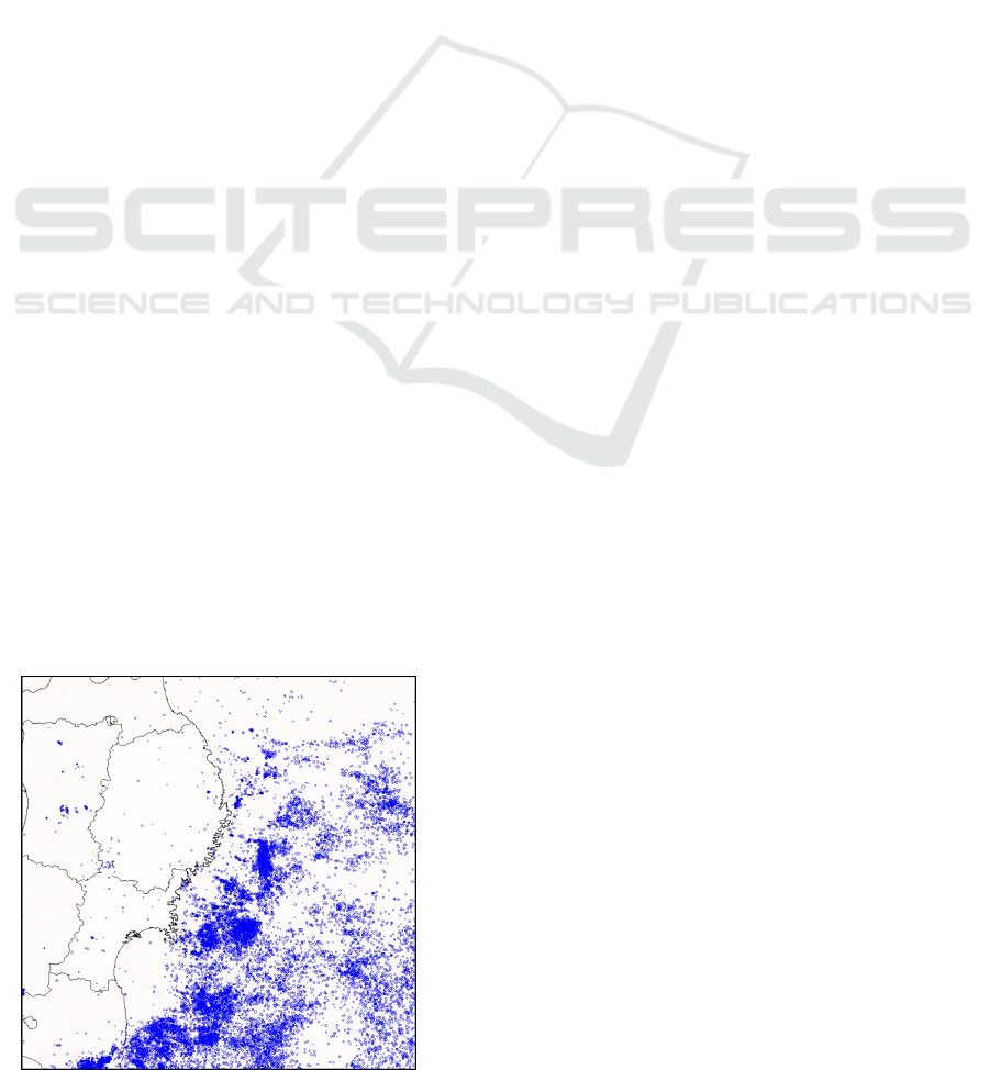
Figure 1: Seismic Activity in Eastern Japan in 2011. Each

circle represents one earthquake.

earthquakes such as Sumatra (2004), Kashmir (2005),

Sichuan (2008) and Touhoku (2011, shown in Fig-

ure 1) caused terrible amounts of casualties.

It is crucially important to understand the pat-

terns and mechanisms behind the occurrence of earth-

quakes. This knowledge may allow us to create bet-

ter seismic risk forecast models, indicating which re-

gions show a higher probability of earthquake occur-

rence at certain periods in time. Such information can

be put to good use for mitigating damage through ur-

ban planning, civil engineering codes, emergency pre-

paredness, et cetera.

Earthquake “prediction” is a polemic subject. No

research so far has even come close to suggesting that

individual large scale earthquakes can be predicted

with any sort of precision. On the other hand, it is

clear that at the very least earthquakes do cluster in

time and space. There is a lot of value behind the

study of earthquake mechanisms, with the goal of

generating statistical models of earthquake risk (Sae-

gusa, 1999). Accordingly, in this paper we focus on

models of earthquake risk, and not on earthquake pre-

diction.

Surprisingly enough, applications of Evolution-

ary Computation (EC) for the problem of earthquake

Aranha C., Lavinas Y., Ladeira M. and Enescu B..

Is it Possible to Generate Good Earthquake Risk Models Using Genetic Algorithms?.

DOI: 10.5220/0005072600490058

In Proceedings of the International Conference on Evolutionary Computation Theory and Applications (ECTA-2014), pages 49-58

ISBN: 978-989-758-052-9

 2014 SCITEPRESS (Science and Technology Publications, Lda.)

forecasting have been few and far between. Given that

EC has some times managed to ﬁnd better solutions

than humans for hard problems (Koza et al., 2003),

we wonder if Artiﬁcial Evolution might not be able

to ﬁnd new ideas that improve our understanding of

earthquakes and their processes.

With this in mind, the goal of this paper is to ex-

plore the suitability of Evolutionary Computation to

the problem of generating earthquake forecast mod-

els. We aim to provide two main contributions:

1. Outline the earthquake forecast problem, which

can be used as a foundation for other researchers

who wish to contribute to this ﬁeld.

2. Show that Evolutionary Computation is a promis-

ing methodology for the creation of earthquake

forecast models, providing the motivation for fur-

ther research in this direction.

It is important to note that our goal is not to gen-

erate an “earthquake alarm system”. Rather, we use

Evolutionary Algorithms to ﬁnd patterns that can be

useful for further understanding the mechanisms be-

hind earthquake occurrence.

A common problem with applications of evolu-

tionary algorithms is how to compare different meth-

ods, developed by different groups with different test-

ing protocols, in a scientiﬁc fashion. We survey and

summarize the “best practices” for the studying and

testing of earthquake forecast models, as suggested

by the Collaboratory for the Study of Earthquake

Predictability (CSEP), an international partnership to

promote rigorous study of the feasibility of earth-

quake forecasting and predictability.

Based on this framework, we design and imple-

ment a simple Genetic Algorithm for earthquake fore-

cast modeling (GAModel). We compare forecasts

generated by the GAModel with the Relative Inten-

sity algorithm (RI) and an information-less forecast.

These systems are applied on the earthquake catalog

from the Japanese Meteorological Agency (JMA), us-

ing event data from 2005 to 2012. The forecasts are

analyzed by their log-likelihood values compared to

the actual data, as suggested in the Regional Earth-

quake Likelihood Model (RELM), and by the Area

Skill Score (ASS) test.

The forecasts created by the GAModel were gen-

erally competitive in relation to the RI algorithm, spe-

cially in scenarios with large amount of inland seis-

mic activity. We discuss some of the strong and weak

points identiﬁed from the experiment. The results

overall show that while there is vast room for im-

provement, Evolutionary Algorithm approaches def-

initely have potential in this ﬁeld.

This paper is an extension of the ideas initially

proposed in (Aranha and Enescu, 2014). In the cur-

rent work, we show the set-up of the genetic algo-

rithm used in great detail, including the discussion of

two ﬁtness function. A larger number of earthquake

scenarios is considered, with the addition of offshore

earthquakes. We also make a detailed presentation

of the problem, to those researchers not familiar with

this ﬁeld.

The paper is organized as follows: in Section 2

we detail the earthquake forecast problem, and the

CSEP framework. Section 3 reviews applications of

Evolutionary Computation in the context of seismol-

ogy research. In Section 4 we detail the proposed

Genetic Algorithm system for generating earthquake

forecasts. In Section 5 we present the results of the

comparisons between this system and the RI algo-

rithm. In Section 6 we discuss the implications of the

results and conclude the paper.

2 THE EARTHQUAKE

FORECASTING PROBLEM

In the ﬁeld of seismology, there is a large number of

model proposals for earthquake forecasting. These

proposals range from methods based on geophysical

principles to purely statistical algorithms.

In this context, the Collaboratory for the Study

of Earthquake Predictability (CSEP)

proposes a

methodology for rigorous scientiﬁc testing of these

many different models.

This testing happens mainly in the shape of dis-

tributed virtual laboratories (Nanjo et al., 2011). Mul-

tiple research groups will submit their forecast mod-

els. These models are be compared against future

earthquake event data using standardized testing pro-

tocols. The testing suite used in these comparisons

is made publicly available by the CSEP, so that re-

searchers can develop and test their models before-

hand.

In many application domains, the lack of an uni-

ﬁed testing protocol means that comparing methods

developed by different research groups can be a great

burden. The CSEP framework allows us to objec-

tively and consistently compare our proposed algo-

rithms with previous approaches.

2.1 Earthquake Forecast Model

In the CSEP framework, a forecast exists in reference

to a geographical region, a start date and an end date.

The forecast will estimate the number (and sometimes

http://www.cseptesting.org

ECTA2014-InternationalConferenceonEvolutionaryComputationTheoryandApplications

Figure 2: Target area for the Kanto region and its bins.

the magnitude) of earthquakes that happens in the tar-

get region during the target time interval.

A forecast is divided into bins. Each bin repre-

sents a non-overlapping geographical interval within

the target region, and sometimes also a magnitude in-

terval.

For example, in this paper we deﬁne the “Kanto”

region as as the area covered by latitude N34.8 to

N36.3, and longitude E138.8 to E140.3. This area is

divided into 2025 bins (a grid of 45x45 squares). Each

bin has an area of approximately 25km

(Figure 2).

For each bin in the forecast we deﬁne a number of

expected earthquakes. This number must be a positive

integer. A good forecast is one where the number of

estimated earthquakes in each bin corresponds to the

actual number of earthquakes that occurs in that bin

during the target time interval.

2.2 Comparison Testing

The CSEP framework uses six different tests to com-

pare earthquake forecasts. These are divided into two

groups: log-likelihood based tests, and alarm based

tests.

The ﬁrst group is based on the analysis of the sim-

ilarity between the forecast and the actual earthquake

catalog, following the Regional Earthquake Likeli-

hood Model (RELM) (Schorlemmer et al., 2007). The

log likelihood of the forecast, given the actual data, is

calculated using a Poisson’s probability distribution.

From this data, three tests are deﬁned. The L-test

compares the difference between the log-likelihood

of the forecast against the actual data, and the log-

likelihood of the forecast against itself. The N-test

tests whether the forecast is predicting too many or

too few events in total, and the R-test provides an al-

gorithm for the statistical testing of multiple forecasts

at once.

These tests require that all forecasts under com-

parison have the same number and size of bins. Also,

due to the way the log likelihood is calculated, they

pose a restriction on the forecast: if any one bin in the

forecast has zero earthquakes, while the correspond-

ing bin in the data has one or more events, the entire

forecast is discarded.

Alarm based tests, on the other hand, use a thresh-

old analysis (Zechar and Jordan, 2010). For a given

forecast a numerical threshold is decided: all bins

with forecast values above the threshold are added to

an alarm set. Earthquakes that fall in this alarm set are

counted as hits, while those falling outside the alarm

set are counted as misses. Alarm based tests rely on

two values: a miss rate v, the proportion of misses to

the total number of earthquakes; and the coverage rate

τ, the smallest alarm set necessary to achieve v.

Three alarm based tests are deﬁned. The Molcham

Diagram draws a path of v and τ based on varying

values of the threshold. The Area Skill Score (ASS) is

deﬁned as the area of the curve under the Molcham

diagram, and can be used to summarize the informa-

tion from the Molcham diagram as a single number.

Finally, a Receiver Operation Characteristic (ROC)

analysis can be done from v and τ. Alarm based tests

can compare forecasts with different bin sizes, but

they do not directly take into account the total number

of earthquakes on the forecast, or the data.

3 EVOLUTIONARY

COMPUTATION FOR

EARTHQUAKE RISK

ANALYSIS

Reports of the application of Evolutionary Computa-

tion and related methods for the generation of earth-

quake forecasts are rather sparse. One such approach

is described by Zhang and Wang (Zhang and Wang,

2012). They use Genetic Algorithms to ﬁne tune an

Artiﬁcial Neural Network (ANN), and use this sys-

tem to produce a forecast. Unfortunately that paper

did not provide enough information to reproduce the

proposed GA+ANN system or their results. Zhou and

Zu (Zhou and Zhu, 2014) also recently proposed a

combination of ANN and EC, but their system only

forecasts the magnitude parameter of earthquakes.

On the other hand, there are quite a few works

using Evolutionary Computation methods for the es-

IsitPossibletoGenerateGoodEarthquakeRiskModelsUsingGeneticAlgorithms?

timation of parameter values in seismological mod-

els. These models are used to describe and understand

particular characteristics of earthquakes or earthquake

activity.

For example, there are many examples of us-

ing Evolutionary Computation to estimate the peak

ground acceleration of seismically active areas (Ker-

mani et al., 2009; Cabalar and Cevik, 2009; Kerh

et al., 2010). Ramos (Ramos and V

azques, 2011)

used Genetic Algorithms to decide the location of

sensing stations in a seismically active area in Mex-

ico. Nicknam et al. (Nicknam et al., 2010) and Ken-

nett and Sambridge (Kennet and Sambridge, 1992)

used evolutionary computation to determine the Fault

Model parameters (such as epicenter location, strike,

dip, etc) of a given earthquake.

4 A FORECAST MODEL USING

GENETIC ALGORITHMS

To investigate the ability of Evolutionary Computa-

tion to generate earthquake forecast models, we de-

sign and test a simple Genetic Algorithm. We call

this system the GAModel.

An individual’s genome in GAModel encodes a

forecast model as deﬁned in the CSEP framework (see

Section 2.1). The population is trained on earthquake

occurrence data for a ﬁxed training period, which is

anterior to the target test period. After the stopping

criterion is reached, the best individual is taken as the

ﬁnal forecast.

By encoding the entire forecast as the genome of

one individual, we identify two concerns that must be

addressed by any EC-based approach: First, as fore-

cast models normally include a few thousand bins,

an individual’s genome will be correspondingly large.

Evolutionary operators and parameters must be cho-

sen to guarantee convergence in a reasonable time

frame.

Second, the design of the ﬁtness function deserves

a lot of attention, to avoid the risk of over ﬁtting the

system to the training data.

4.1 Genome Representation

In GAModel, each individual represents an entire

forecast model. The genome is a real valued array

X, where each element corresponds to one bin in the

desired model (the number of bins n is deﬁned by the

problem). Each element x

∈ X takes a value from

[0,1). In the initial population, these values are sam-

pled from a uniform distribution.

In the CSEP framework, a model is deﬁned as a set

of integer valued expectations, corresponding to the

number of earthquakes for each bin. To convert from

the real valued chromosome to a integer forecast, we

use a modiﬁcation of the Poisson deviates extraction

algorithm from (Press et al., 2007) (Chapter 7.3.12).

Algorithm 1: Obtain a Poisson deviate from a [0,1)

value.

Parameters 0 ≤ x < 1,µ ≥ 0

L ← exp(−µ),k ← 0, prob ← 1

repeat

increment k

prob ← prob ∗ x

until prob > L

return k

In Algorithm 1, x is the real value taken from

the chromosome, and µ is the average number of

earthquakes observed across the entire training data.

Note that in the original algorithm, k − 1 is re-

turned. Because the log likelihood calculation used

for model comparison discards forecasts that estimate

zero events in bins where earthquakes are observed,

we modify the original algorithm to make sure all bins

estimate at least one event.

4.2 Fitness Function

Usually, the main challenge when applying an Evolu-

tionary Computation method to any new application

domain is the deﬁnition of an appropriate ﬁtness func-

tion. Accordingly, a large part of our effort was used

to deﬁne a good ﬁtness function for GAModel.

We describe two candidate ﬁtness functions. The

ﬁrst one is a direct application of the log likelihood

deﬁnition for earthquake forecast. Because this ﬁt-

ness function resulted in an excessive amount of over

ﬁtting, we describe a second ﬁtness function that

breaks the training data set into smaller data sets in

order to avoid this problem.

4.2.1 Simple Log Likelihood Fitness Function

This ﬁtness function uses the log-likelihood between

the forecast generated by an individual and the ob-

served earthquakes in the training data, as described

by Schorlemmer et al. (Schorlemmer et al., 2007). In

simple terms, the log likelihood is a measure of how

close a forecast is to a given data set.

Let Λ = {λ

,λ

,. .. ,λ

|λ

∈ N} be a forecast with

n bins. In this deﬁnition, λ

is the number of earth-

quakes that is forecast to happen in bin i. To derive

from an individual X = {x

,. .. ,x

|0 ≤ x

< 1},

we calculate each λ

from x

using Algorithm 1.

ECTA2014-InternationalConferenceonEvolutionaryComputationTheoryandApplications

Now, let Ω = {ω

,ω

,. .. ,ω

|ω

∈ N} be the ob-

served numbers of earthquakes for each bin i in the

training data. The log likelihood between an individ-

ual’s forecast Λ

and the observed data Ω is calcu-

lated as:

L(Λ

|Ω) =

∑

i=0

−λ

+ ω

∗ ln(λ

) − ln(ω

!) (1)

There are two special cases that arise when any λ

= 0.

If λ

= 0 and ω

= 0, then the value of the sum for that

element is 1. If ω

> 0, then L(Λ

|Ω) = −∞ and the

forecast must be discarded. For more details on this,

see (Schorlemmer et al., 2007).

In the Simple Log Likelihood ﬁtness function, the

value of L(Λ

|Ω) is taken directly as the ﬁtness value

of the individual.

Early testing with the Simple Log Likelihood

function showed that GAModel had a very strong ten-

dency to over ﬁt to the training data. This is natural,

since there are differences between the seismicity of a

larger period and a shorter one. To solve this problem,

we used the ﬁtness function shown in the next section.

4.2.2 Time-slice Log Likelihood Fitness

Function

In the time-slice log likelihood ﬁtness function we

break up the training data set into smaller slices.

These slices are based on the chronology of the earth-

quakes contained in the training catalog. The duration

of each slice is the same as the duration of the target

interval (the test data).

Let’s consider an example: the target period for

the forecast is one year, from 1/1/2014 to 1/1/2015,

and the training data is taken from the 10 year pe-

riod between 1/1/2004 and 1/1/2014. To apply the

time-slice log likelihood ﬁtness function, we divide

the training data into ten 1-year slices, from 2004 to

2005, 2005 to 2006, and so on.

When an individual X is evaluated, we calculate

the log likelihood of its forecast Λ

against each of

the time slices (Ω

2004

,Ω

2005

,. .. ,Ω

2013

). We use the

lowest log likelihood value from among all the slices

as the ﬁtness value of X.

The idea behind this ﬁtness function is that the cat-

alog data available for training will normally span a

period of time much longer than the desired forecast.

By breaking the training data into smaller periods, we

are trying to make the evolutionary algorithm learn

any time-repeating pattern that might exist in the data.

We choose the smallest log likelihood from the time

slices in order to make sure that the evolution process

favors solutions that try to solve all slices equally.

4.3 Evolutionary Operators and

Parameters

GAModel uses a regular generational genetic algo-

rithm. For selection, we use Elitism and Tournament

selection.

We use a simple Uniform Crossover for the

crossover operator. If a gene’s value falls outside the

[0,1) boundary, it is truncated to these limits. For

the mutation operator, we sample entirely new values

from [0,1) for each mutated chromosome.

Table 1: Parameters used in GAModel.

Population Size 500

Generation Number 100

Elite Size 1

Tournament Size 50

Crossover Chance 0.9

Mutation Chance (individual) 0.8

Mutation Chance (chromosome) (genome size)

−1

The parameters used for the evolutionary compu-

tation are described in Table 1. Because our focus is

to show the viability of Evolutionary Algorithms for

this application problem, we are not yet particularly

concerned with the convergence speed of the system.

Accordingly, not a lot of effort was spent ﬁne tuning

these parameter values. These values were chosen in-

stead by trial and error on a data region not used in the

experiments of Section 5.1, until an acceptable con-

vergence time was found.

It would be very interesting to perform an ex-

tended effort into identifying the sensibility of each

parameter above to the current application domain.

For example, while in this work we are worried about

analyzing the inﬂuence of the ﬁtness function in the

degree of over ﬁtting in the results, a precise control

of the value for the tournament size parameter might

also have an effect in this regard.

5 EXPERIMENTS

To analyze the performance of the forecasts gener-

ated by the GAModel, we execute a simulation ex-

periment. In this simulation, the GAModel evolves

using a training data set, and the resulting forecast

is analyzed against a test data set. These results are

compared against two other forecasts: an “unskilled”

model, which randomly guesses the forecast (Fig-

ure 4), and a forecast generated by the Relative In-

tensity (RI) algorithm, regarded as a natural reference

for comparative tests with earthquake forecast mod-

els (Nanjo, 2011).

IsitPossibletoGenerateGoodEarthquakeRiskModelsUsingGeneticAlgorithms?

5.1 Experimental Data

The data used in these experiments comes from the

Japan Meteorological Agency’s (JMA) catalog. The

catalog lists earthquakes recorded by the sensing sta-

tion network in Japan. For each earthquake, the fol-

lowing values are given: time of occurrence, magni-

tude, latitude and longitude and depth of the hypocen-

ter.

To avoid issues related to the incompleteness of

the catalogue for very weak or very deep earthquakes,

we consider only events with magnitude above 2.5

and depth less than 100km. We consider earthquakes

recorded in the period between 2000 and 2013. This

accounts for more than 220.000 earthquakes in the

Japanese archipelago.

To achieve a better understanding of the forecast-

ing power of GA models, we deﬁne four areas (sce-

narios) to focus in our experiment. Figure 3 shows

where these four areas are located within Japan.

Three of these areas (Kanto, Touhoku and Kansai),

contain mainly inland earthquakes, which are con-

sidered to follow more stable patterns. The fourth

area (East Japan) includes also many off-shore earth-

quakes. To make it easier to compare the results for

each area, we choose the bin size so that the total

number of bins is within the same order of magnitude

in all areas.

1. Kanto: Kanto is the area at and nearby Tokyo.

There is a large amount of seismic activity in the

target period. In this study, we deﬁne this region

as starting at N34.8,W138.8, with 2025 bins ar-

ranged in a 45x45 grid. Each bin corresponds to a

square with 25km

2. Kansai: The Kansai area includes Kyoto, Osaka,

Kobe and nearby cities. This area shows a rela-

tively lower amount of seismic activity in the pe-

riod considered. We deﬁne this region as start-

ing at N34,W134.5, with 1600 bins arranged in

a 40x40 grid. Each bin corresponds to a 25km

square.

3. Touhoku: The Touhoku region is deﬁned as the

northern provinces of the main island. It shows

some clusters of seismic activity during the pe-

riod studied. We deﬁne this region as starting at

N37.8,W139.8, with 800 bins arranged in a 40x20

grid. Each bin corresponds to a 100km

square.

4. East Japan: This area corresponds to Japan’s

north-eastern coast. It includes both inland and

off-shore events, which makes it more difﬁcult to

forecast. It also includes the location of the M9

earthquake of 2011. We deﬁne this region as start-

ing at N37,W140, with 1600 bins arranged in a

Figure 3: The relative locations of the four areas used in our

experiments.

40x40 grid. Each bin corresponds to a 100km

square.

5.2 Experimental Design

To compare the performance of the different fore-

cast models, we execute a simulation experiment on

32 scenarios. A scenario is deﬁned by a target re-

gion and a target time interval. The region is selected

from the four regions described in the previous sec-

tion. The time interval is a one year interval, lasting

from Jan/01 to Dec/31. We consider 8 periods (from

2005 to 2012). In each period, we use 5 years of prior

data (2000 to 2011) to train the RI and GAM algo-

rithms.

For each scenario, we generate forecasts for the

random model, the GAM model (using the second

ﬁtness function described in this paper) and the RI

model. The random forecast is generated by selecting

a random uniform value between 0 and 1 for each bin,

and transforming this value into an integer using Al-

gorithm 1. The RI forecast is generated according to

Section 5.3.

Both the GAModel and the RI algorithm require

a training data set. For each scenario, we use earth-

quake data from the 5 year period immediately prior

to the testing period. In order to test the statistical

signiﬁcance of our results, we run the GAModel 20

times, and obtain 20 forecasts. All GAModel results,

unless noted otherwise, are the mean of these 20 runs.

Because the RI algorithm is not stochastic, the result

of a single run is reported.

The results are compared in mainly two ways. We

report the log likelihood values for the three methods.

The log likelihood indicates how close the forecast

ECTA2014-InternationalConferenceonEvolutionaryComputationTheoryandApplications

Figure 4: A random forecast (Kansai Region, 2007).

is to the test data, in terms of location and quantity

of earthquakes. We also report the Area Skill Score

(ASS) for the three methods. The ASS is the area

covered by the “Alarm rate x Miss rate” curve of the

forecast (see Section 2.2 for details). In both cases, a

higher value indicates a more skilled model.

5.3 The Relative Intensity Algorithm

The Relative Intensity (RI) algorithm is a commonly

used benchmark for earthquake forecasting models.

In this experiment, we use it as goalpost to assess the

suitability of evolutionary computation for earthquake

forecasting.

The working assumption behind the RI is that

larger earthquakes are more likely to occur at loca-

tions of high seismicity in the past. Accordingly,

the RI algorithm will estimate the number of earth-

quakes in a bin based on the number of earthquakes

observed in the past for that bin. This estimate will be

“smoothed” by an attenuation factor s that takes into

account the seismicity of neighboring bins.

We use the implementation described by Nanjo

in (Nanjo, 2011). Please refer to that paper for im-

plementation details. The parameters used for the

RI algorithm in these experiments are: b = 0.8 and

s = 50km. These values were selected by taking the

suggested range of values recommended in (Nanjo,

2011), and ﬁnding the best values in this range on the

same data set used to tune the parameters of the Ge-

netic Algorithm.

5.4 Comparison of Forecast Models

The results of the simulation experiments are summa-

rized in Table 2. In this table, Random refers to the

Random forecast, RI to the Relative Intensity algo-

rithm, and GA to the GAModel.

The GA column reports the average for 20 runs,

and the standard deviation is reported in parenthesis.

The p-value column indicates the result of an one-

sided T-test of the GA’s mean against the value ob-

tained from the RI algorithm.

Looking at the table, we observe that the

GAModel has generally outperformed the RI on the

“Kanto” area. Figures 5(c) and 5(d) illustrate the rea-

son: Generally, GAModel is able to detect smaller

earthquake clusters inland, while RI smooths them

out.

Even then, both models miss some clusters in this

area, as indicated by their ASS value being under the

value of the random model. The ASS value is useful

to estimate how much a forecast is suffering from over

ﬁtting - a low value indicates that a larger alarm area

is necessary to reduce the miss rate of the forecast.

The “Touhoku” area shows a similar situation as

the “Kanto” area. In Figures 5(a) and 5(b) we can

see that GAModel is able to identify the two earth-

quake clusters more precisely, while the RI algorithm

casts a wide net which reduces the forecast accuracy.

The ASS score for this area is higher. This is because

both methods are able to learn the two “hot spots” for

seismic activity, unlike the Kanto area where some

clusters would appear in different locations along the

years.

Conversely, in the “East Japan” area the RI algo-

rithm performed better than the GAModel. The rea-

son seems to be that off-shore seismicity, which is

spread over a larger area than inland events, is better

captured by the wide smoothing step of the RI algo-

rithm.

In all three cases, we can see that the results

changed wildly in the aftermath of the 2011 M9 earth-

quake. That earthquake caused a sudden large spike

of seismic activity in all areas (Figure 1), includ-

ing many areas that never showed any seismic ac-

tivity during the training period. In the following

scenario (2012), both methods try to use this new

data to reform their forecasts. Again, GAModel per-

forms better in the “Touhoku/2012” scenario, where

most earthquakes are inland. The RI method per-

forms better in the “Kanto/2012” scenario, where

most of the new seismicity occurs off-shore (Fig-

ures 5(e) and 5(f)).

The “Kansai” scenarios turned out to be a special

situation for both algorithms. The seismic activity in

that area for the period was too sparse. Since both

the RI and GAModel depend on the analysis of re-

cent earthquakes, neither algorithm could produce a

reliable forecast. In the case of the RI, the forecast

IsitPossibletoGenerateGoodEarthquakeRiskModelsUsingGeneticAlgorithms?

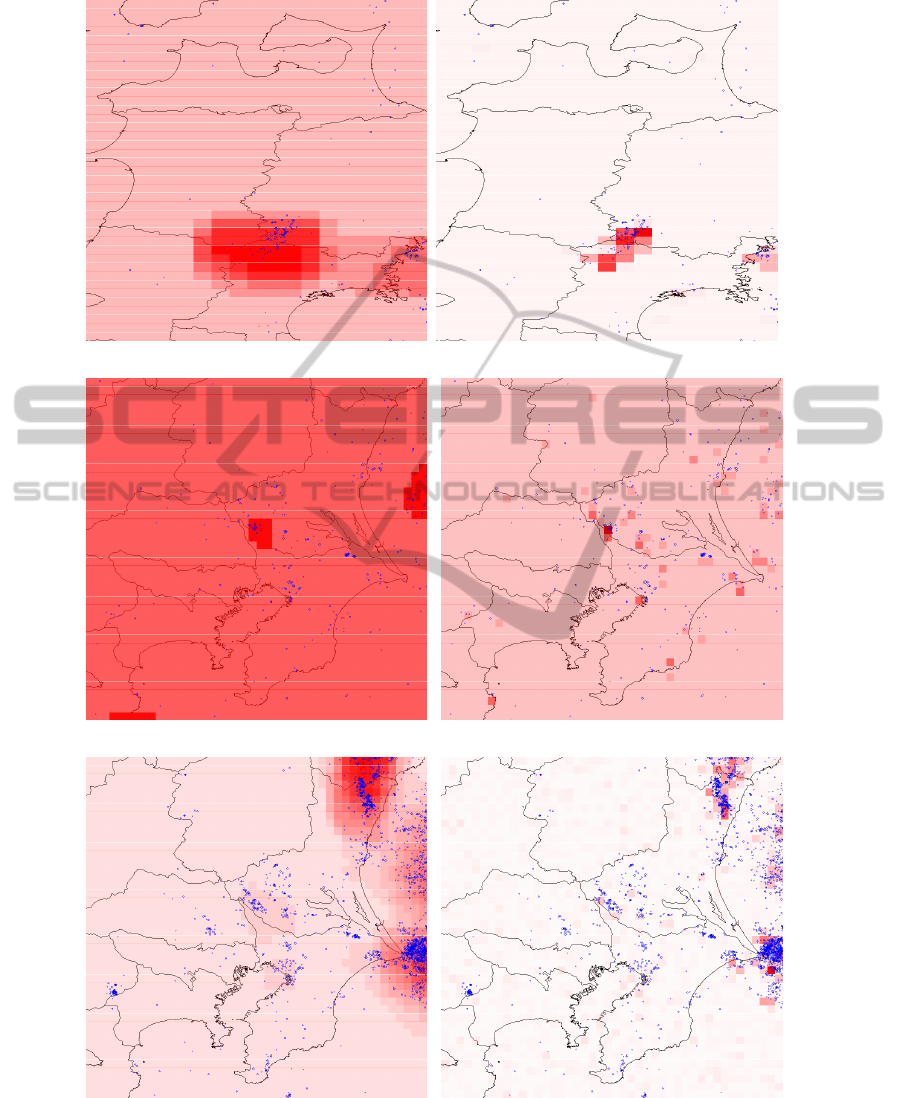
(a) Touhoku 2009, RI forecast (b) Touhoku 2009, GA forecast

(e) Kanto 2012, RI forecast (f) Kanto 2012, GA forecast

Figure 5: Some forecast images for the RI algorithm and the GAModel. Red squares indicate the intensity of the forecast.

Blue circles indicate actual earthquakes in the test data. Note that the intensity of the red color indicates relative values in

the forecast. In other words, uniform forecasts will tend to appear as a darker red color than forecasts with a bigger range of

values.

ECTA2014-InternationalConferenceonEvolutionaryComputationTheoryandApplications

Table 2: Results from the simulation experiments. The parenthesis after the GA values are the standard deviation (average of

20 runs). The two “p-value” columns report the signiﬁcance of the t-test comparing the GA mean against the result from the

RI algorithm. For the sake of legibility, p-values under 0.01 are reported as 0.01.

Scenario Log Likelihood Area Skill Score

Random RI GA p-value Random RI GA p-value

Kanto 2005 -3716.86 -2263.4 -2253.2 (16.5) 0.01 0.38 0.24 0.24 (0.04) 0.78

2006 -3884.85 -2252.28 -2234.72 (14) 0.01 0.36 0.10 0.18 (0.01) 0.01

2007 -3838.9 -2113.84 -2108.95 (11.1) 0.03 0.36 0.15 0.19 (0.02) 0.01

2008 -3914.54 -2110.79 -2096.75 (11.8) 0.01 0.39 0.16 0.22 (0.03) 0.01

2009 -4211.28 -2487.88 -2482.88 (10.3) 0.02 0.36 0.09 0.14 (0.01) 0.01

2010 -4010.47 -2132.11 -2099.13 (16.3) 0.01 0.39 0.14 0.28 (0.03) 0.01

2011 -17657.43 -20083.09 -19983.73 (144.4) 0.01 0.35 0.07 0.08 (0.02) 0.14

2012 -10863.99 -3225.39 -4435.34 (248) 1.00 0.48 0.80 0.77 (0.01) 1.00

Kansai 2005 -2219.06 -1605 -1631.96 (26) 0.99 0.24 0 0.07 (0.02) 0.01

2006 -2172.29 -1606 -1631.19 (23.9) 0.99 0.23 0 0.05 (0.01) 0.01

2007 -2024.77 -1615 -1617.01 (2.3) 0.99 0.22 0 0.03 (0.01) 0.01

2008 -2038.16 -1608 -1610.41 (1.54) 1.00 0.22 0 0.01 (0.01) 0.01

2009 -2054.23 -1618 -1619.51 (2.58) 0.99 0.21 0 0.02 (0.01) 0.01

2010 -2054.63 -1613 -1611.00 (2.27) 0.01 0.27 0 0.07 (0.02) 0.01

2011 -2059.89 -1625 -1625.12 (2.46) 0.58 0.26 0 0.05 (0.03) 0.01

2012 -2080.35 -1601 -1603.59 (2.92) 0.99 0.22 0 0.04 (0.02) 0.01

Touhoku 2005 -2552.61 -1067.38 -984.23 (84) 0.01 0.58 0.58 0.62 (0.01) 0.01

2006 -2613.1 -1044.72 -1073.03 (154) 0.78 0.52 0.50 0.42 (0.03) 1.00

2007 -2666.11 -1049.82 -999.64 (83.6) 0.01 0.51 0.51 0.41 (0.01) 1.00

2008 -5124.54 -5007.49 -4704.15 (131) 0.01 0.36 0.05 0.18 (0.01) 0.01

2009 -2737.47 -1049.22 -936.63 (60) 0.01 0.54 0.67 0.70 (0.01) 0.01

2010 -2714.68 -1045.03 -1077.95 (136) 0.85 0.53 0.66 0.57 (0.01) 1.00

2011 -3435.67 -2753.95 -2963.31 (88) 1.00 0.40 0.21 0.10 (0.01) 1.00

2012 -3623.22 -1326.52 -1186.1 (45.3) 0.01 0.47 0.62 0.70 (0.05) 0.01

East Japan 2005 -2666.11 -1049.82 -868.87 (20) 0.01 0.47 0.35 0.30 (0.02) 1.00

2006 -6596.76 -2130.69 -2303.78 (98) 1.00 0.46 0.42 0.35 (0.01) 1.00

2007 -6714.36 -1997.78 -2065.4 (85) 0.99 0.43 0.51 0.34 (0.02) 1.00

2008 -8784.64 -6087.88 -6097.63 (264) 0.56 0.46 0.23 0.20 (0.03) 1.00

2009 -6435.07 -2052.35 -1964.72 (106) 0.01 0.47 0.49 0.48 (0.02) 0.99

2010 -6560.97 -2572.97 -2541.33 (121) 0.12 0.46 0.41 0.31 (0.01) 1.00

2011 -31447.79 -47704.35 -51485.77 (536) 1.00 0.44 0.40 0.18 (0.01) 1.00

2012 -19068.86 -5177.55 -6657.52 (478) 1.00 0.50 0.77 0.71 (0.01) 1.00

produced was largely a uniform forecast, where all

bins had equal or very close expectation values. In

the case of GAModel, A few bins where earthquakes

had happened in the training data were marked with

higher forecasts, but no consistent activity clusters

were identiﬁed. The log likelihood or ASS scores for

these scenarios cannot really be used to compare the

two methods.

6 CONCLUSION

Our goal in this work was to open the discussion

about the feasibility of Evolutionary Computation

approaches for the important problem of generat-

ing earthquake forecast models. The mechanisms of

earthquake generation are still not fully understood,

which motivates us to use self-adaptive methods such

as Genetic Algorithms.

To illustrate our proposal, we designed GAModel,

a traditional GA with an speciﬁc ﬁtness function that

generates an earthquake forecast based on recent seis-

mic history. We performed simulation experiments

and compared the results with the RI method, which

is accepted in the seismology community as a natural

benchmark.

Our results show that the GAModel is competi-

tive with the RI algorithm, outperforming it in scenar-

ios with a predominance of in-land earthquakes, and

being outperformed when there is a large number of

off-shore earthquakes. In this sense, we feel that the

answer to the question posed by the title of the paper

should be “Yes, it is promising to use EC to generate

earthquake forecasts”.

That said, we have also identiﬁed many places

where an Evolutionary forecast generator could be

improved. Although the time-slice ﬁtness function

was designed to reduce over ﬁtting, we still see that

IsitPossibletoGenerateGoodEarthquakeRiskModelsUsingGeneticAlgorithms?

GAModel generates “sharp” forecasts that are proba-

bly the result of some degree of over ﬁtting.

In this paper, we have decided to focus on the in-

troduction of this new problem domain to the evo-

lutionary computation community. Therefore, we

limited ourselves to the traditional GA. However,

we visualize many possible research directions based

on the shortcomings demonstrated in the current re-

search.

One way to mitigate the sharpness noticed in the

results is by making the algorithm aware of data lo-

cality. Based on the smoothing pattern in the RI al-

gorithm, we plan to develop a self-adaptive way to

smooth the results in the GAM. Also, because in the

RELM each bin is ultimately evaluated independently

of the neighboring bins, it is feasible to imagine that

separate areas in a forecast model could be generated

by using different parameters, or different algorithm

variations altogether.

Finally, we currently only use historical data to

build the forecast model. We are very interested in

ﬁnding ways to add domain knowledge into the sys-

tem, such as the location of known faults, in order to

improve the forecast ability.

ACKNOWLEDGEMENTS

We would like to thank the Japan Meteorological

Agency for the earthquake catalog used in this study.

REFERENCES

Aranha, C. and Enescu, B. (2014). A study on the viability

of evolution methods for the generation of earthquake

predictability models. In The 28th annual conference

of the Japan Society on Artiﬁcial Intelligence.

Cabalar, A. F. and Cevik, A. (2009). Genetic programming-

based attenuation relationship: An application of re-

cent earthquakes in Turkey. Computers and Geo-

sciences, 35:1884–1896.

Kennet, B. L. N. and Sambridge, M. S. (1992). Earthquake

location genetic algorithms for teleseisms. Physics of

the Earth and Planetary Interiors, 75(1–3):103–110.

Kerh, T., Gunaratnam, D., and Chan, Y. (2010). Neural

computing with genetic algorithm in evaluating poten-

tially hazardous metropolitan areas result from earth-

quake. Neural Comput. Appl., 19(4):521–529.

Kermani, E., Jafarian, Y., and Baziar, M. H. (2009). New

predictive models for the v

max

ratio of strong

ground motions using genetic programming. Interna-

tional Journal of Civil Engineering, 7(4):236–247.

Koza, J. R., Keane, M. A., and Streeter, M. J. (2003).

What’s AI done for me lately? Genetic program-

ming’s human-competitive results. IEEE Intelligent

Systems, 18(3):25–31.

Nanjo, K. Z. (2011). Earthquake forecasts for the CSEP

Japan experiment based on the RI algorithm. Earth

Planets Space, 63:261–274.

Nanjo, K. Z., Tsuruoka, H., Hirata, N., and Jordan, T. H.

(2011). Overview of the ﬁrst earthquake forecast

testing experiment in Japan. Earth Planets Space,

63:159–169.

Nicknam, A., Abbasnia, R., Eslamian, Y., Bozorgnasab, M.,

and Mosabbeb, E. A. (2010). Source parameters esti-

mation of 2003 Bam earthquake Mw 6.5 using empiri-

cal Green’s function method, based on an evolutionary

approach. J. Earth Syst. Sci., 119(3):383–396.

Press, W. H., Teukolsky, S. A., Vetterling, W. T., and Flan-

nery, B. P. (2007). Numerical Recipes, The Art of Sci-

entiﬁc Computing. Cambridge University Press, third

edition.

Ramos, J. I. E. and V

azques, R. A. (2011). Locat-

ing seismic-sense stations through genetic algorithms.

In Proceedings of the GECCO’11, pages 941–948,

Dublin, Ireland. ACM.

Saegusa, A. (1999). Japan tries to understand quakes, not

predict them. Nature, 397:284–284.

Schorlemmer, D., Gerstenberger, M., Wiemer, S., Jackson,

D., and Rhoades, D. A. (2007). Earthquake likeli-

hood model testing. Seismological Research Letters,

78(1):17–29.

Zechar, J. D. and Jordan, T. H. (2010). The area skill

score statistic for evaluating earthquake predictability

experiments. Pure and Applied Geophysics, 167(8–

9):893–906.

Zhang, Q. and Wang, C. (2012). Using genetic algorithms

to optimize artiﬁcial neural network: a case study

on earthquake prediction. In Second International

Conference on Genetic and Evolutionary Computing,

pages 128–131. IEEE.

Zhou, F. and Zhu, X. (2014). Earthquake prediction based

on LM-BP neural network. In Liu, X. and Ye, Y., edi-

tors, Proceedings of the 9th International Symposium

on Linear Drives for Industry Applications, Volume 1,

volume 270 of Lecture Notes in Electrical Engineer-

ing, pages 13–20. Springer Berlin Heidelberg.

ECTA2014-InternationalConferenceonEvolutionaryComputationTheoryandApplications