
Pattern Recognition by Probabilistic Neural Networks
Mixtures of Product Components versus Mixtures of Dependence Trees
Jiˇr´ı Grim
1
and Pavel Pudil
2
1
Institute of Information Theory and Automation, Czech Academy of Sciences, Prague, Czech Republic
2
Faculty of Management, Prague University of Economics, Jindˇrich˚uv Hradec, Czech Republic
Keywords:
Probabilistic Neural Networks, Product Mixtures, Mixtures of Dependence Trees, EM Algorithm.
Abstract:
We compare two probabilistic approaches to neural networks - the first one based on the mixtures of product
components and the second one using the mixtures of dependence-tree distributions. The product mixture
models can be efficiently estimated from data by means of EM algorithm and have some practically important
properties. However, in some cases the simplicity of product components could appear too restrictive and a
natural idea is to use a more complex mixture of dependence-tree distributions. By considering the concept of
dependence tree we can explicitly describe the statistical relationships between pairs of variables at the level
of individual components and therefore the approximation power of the resulting mixture may essentially
increase. Nonetheless, in application to classification of numerals we have found that both models perform
comparably and the contribution of the dependence-tree structures decreases in the course of EM iterations.
Thus the optimal estimate of the dependence-tree mixture tends to converge to a simple product mixture model.
Regardless of computational aspects, the dependence-tree mixtures could help to clarify the role of dendritic
branching in the highly selective excitability of neurons.
1 INTRODUCTION
Considering the probabilistic approach to neural net-
works in the framework of statistical pattern recog-
nition we approximate the unknown class-conditional
probability distributions by mixtures of product com-
ponents (Grim, 1996; Grim, 2007). The basic princi-
ple of probabilistic neural networks (PNN) is to view
the mixture components as formal neurons. We have
shown that the component parameters can be esti-
mated by a sequential strictly modular version of EM
algorithm (Grim, 1999b). The estimated mixtures de-
fine an information preserving transform which can
be used to design multilayer PNN sequentially (Grim,
1996). The independently designed information pre-
serving transforms can be combined both in the hori-
zontal and vertical sense (Grim et al., 2002). A sub-
space modification of EM algorithm can be used to
optimize the structure of incompletely interconnected
PNN (Grim et al., 2000). In a series of papers we have
analyzed the properties of PNN in application to prac-
tical problems of pattern recognition (Grim and Hora,
2008).
The probabilistic neuron can be interpreted from
the neurophysiological point of view in terms of the
functional properties of biological neurons (Grim,
2007). In particular the explicit formula for the synap-
tic weight can be viewed as a theoretical counter-
part of the well known Hebbian principle of learn-
ing (Hebb, 1949). The information preserving trans-
form assumes the activation function of probabilistic
neurons in a logarithmic form and, in this way, the
product components define the output of a neuron as
a weighted sum of synaptic contributions. In addition,
the mixtures of product components have some spe-
cific advantages, like easily available marginals and
conditional distributions, a direct applicability to in-
complete data and the possibility of structural opti-
mization of multilayer PNN (Grim, 1986). The con-
cept of PNN is also compatible with the technique of
boosting (Grim et al., 2002b) which can be used to
model emotional learning.
However, there is also a computational motiva-
tion to apply the product mixture model. In the
last decades there is an increasing need of estimat-
ing multivariate and multimodal probability distribu-
tions from large data sets. Such databases are usu-
ally produced by information technologies in vari-
ous areas like medicine, image processing, monitor-
ing systems, communication networks and others. A
65
Grim J. and Pudil P..
Pattern Recognition by Probabilistic Neural Networks - Mixtures of Product Components versus Mixtures of Dependence Trees.
DOI: 10.5220/0005077500650075
In Proceedings of the International Conference on Neural Computation Theory and Applications (NCTA-2014), pages 65-75
ISBN: 978-989-758-054-3
Copyright
c
2014 SCITEPRESS (Science and Technology Publications, Lda.)

typical feature of the arising “technical” data is a
high dimensionality and a large number of measure-
ments. The unknown underlying probability distri-
butions or density functions are nearly always multi-
modal and cannot be assumed in a simple paramet-
ric form. In this sense, one of the most efficient
possibilities is to approximate the unknown multidi-
mensional probability distributions by finite mixtures
and, especially, by mixtures of components defined
as products of univariate distributions (Grim, 1982;
Grim, 1986; Grim et al., 2000; Grim, 2007; Grim and
Hora, 2010; Lowd and Domingos, 2005). In the past
the approximation potential of product mixtures has
been often underestimated probably because of for-
mal similarity with the so-called naive Bayes mod-
els which assume the class-conditional independence
of variables (Lowd and Domingos, 2005). In con-
nection with product mixtures this term is incorrectly
used because there is nothing naive on the assump-
tion of product components of mixtures. In case of
discrete variables the product mixtures are universal
approximators since any discrete distribution can be
expressed as a product mixture (Grim, 2006). Simi-
larly, the Gaussian productmixtures approach the uni-
versality of non-parametric Parzen estimates with the
increasing number of components.
Nevertheless, despite the advantageous properties
of product mixtures, the simplicity of product com-
ponents may become restrictive in some cases. For
this reason it could be advantageous to consider the
mixture components in a more specific form. A nat-
ural approach is to use dependence-tree distributions
(Chow and Liu, 1968) as components. By using the
concept of dependence tree we can explicitly describe
the statistical relationships between pairs of variables
at the level of individual components. Therefore,
the approximation “power” of the resulting mixture
model should increase. We have shown (Grim, 1984)
that mixtures of dependence-tree distributions can be
optimized by EM algorithm in full generality.
In the domain of probabilistic neural networks the
mixtures of dependencetrees could help to explain the
role of dendritic branching in biological neurons. It is
assumed that easily excitable thin dendritic branches
may facilitate the propagation of excitation to neural
body and the effect of conditional facilitation could
be modeled by the dependence-tree structure.
In this paper we describe first the product mixture
model (Sec. 2, Sec. 3). In Sec. 4 we recall the con-
cept of dependence-tree distribution in the framework
of finite mixtures. In Sec.5 we discuss different as-
pects of the two types of mixtures in a computational
experiment - in application to recognition of numer-
als. The results are summarized in the Conclusion.
2 ESTIMATING MIXTURES
Considering distribution mixtures, we approximate
the unknown probability distributions by a linear
combination of component distributions
P(x|w,Θ) =
∑
m∈M
w
m
F(x|θ
m
), (1)
w = (w
1
,w
2
,...,w
M
), θ
m
= {θ
m1
,θ
m2
,. ..,θ
mN
}.
where x ∈ X are discrete or real data vectors, w is the
vector of probabilisticweights, M = {1,.. .,M} is the
component index set and F(x|θ
m
) are the component
distributions with parameters θ
m
.
Since the late 1960s the standard way to esti-
mate mixtures is to use the EM algorithm (Hassel-
blad, 1966; Schlesinger, 1968; Hasselblad, 1969;
Day, 1969; Hosmer, 1973; Wolfe, 1970; Dempster
et al., 1977; Grim, 1982). Formally, given a finite set
S of independent observations of the underlying N-
dimensional random vector
S = {x
(1)
,x
(2)
,. ..}, x = (x
1
,x
2
,. ..,x
N
) ∈ X, (2)
we maximize the log-likelihood function
L(w,Θ) =
1
|S|
∑
x∈S
log
"
∑
m∈M
w
m
F(x|θ
m
)
#
(3)
by means of the following EM iteration equations
(m ∈ M ,n ∈ N ,x ∈ S ):
q(m|x) =
w
m
F(x|θ
m
)
∑
j∈M
w
j
F(x|θ
j
)
, w
′
m
=
1
|S|
∑
x∈S
q(m|x),
(4)
Q
m
(θ
m
) =
∑
x∈S
q(m|x)
∑
y∈S
q(m|y)
logF(x|θ
m
), (5)
θ
′
m
= argmax
θ
m
n
Q
m
(θ
m
)
o
. (6)
Here the apostrophe denotes the new parameter val-
ues in each iteration. One can easily verify (cf. (Grim,
1982)) that the general iteration scheme (4) - (6) pro-
duces nondecreasing sequence of values of the max-
imized criterion (3). In view of the implicit relation
(6) any new application of EM algorithm is reduced
to the explicit solution of Eq. (6).
Considering product mixtures, we assume the
component distributions F(x|θ
m
) defined by products
F(x|θ
m
) =
∏
n∈N
f
n
(x
n
|θ
mn
), m ∈ M (7)
and therefore Eqs. (6) can be specified for variables
independently:
Q
mn
(θ
mn
) =
∑
x∈S
q(m|x)
w
′
m
|S|
log f
n
(x
n
|θ
mn
), (8)
NCTA2014-InternationalConferenceonNeuralComputationTheoryandApplications
66

θ
′
mn
= argmax
θ
mn
n
Q
mn
(θ
mn
)
o
, n ∈ N . (9)
The mixtures of product components have some
specific advantages as approximation tools. Recall
that any marginal distribution of product mixtures is
directly available by omitting superfluous terms in
product components. Thus, in case of prediction,
we can easily compute arbitrary conditional densities
and for the same reason product mixtures can be esti-
mated directly from incomplete data without estimat-
ing the missing values (Grim et al., 2010). Product
mixtures support a subspace modification for the sake
of component-specific feature selection (Grim, 1999;
Grim et al., 2006) and can be used for sequential pat-
tern recognition by maximum conditional informativ-
ity (Grim, 2014). Moreover, the product components
simplify the EM iterations and increase the numerical
stability of EM algorithm.
3 MULTIVARIATE BERNOULLI
MIXTURES
In case of binary data x
n
∈ {0,1} the product mix-
ture model is knownas multivariate Bernoulli mixture
based on the univariate distributions
f
n
(x
n
|θ
mn
) = (θ
mn
)
x
n
(1− θ
mn
)
1−x
n
, 0 ≤ θ
mn
≤ 1,
with the resulting product components
F(x|θ
m
) =
∏
n∈N
(θ
mn
)
x
n
(1− θ
mn
)
1−x
n
, m ∈ M . (10)
The conditional expectation criterion Q
mn
(θ
mn
) can
be expressed in the form
Q
mn
(θ
mn
) =
∑
ξ∈X
n
∑
x∈S
δ(ξ,x
n
)
q(m|x)
w
′
m
|S|
log f
n
(ξ|θ
mn
),
and therefore there is a simple solution maximizing
the weighted likelihood (9):
θ
′
mn
=
∑
x∈S
x
n
q(m|x)
w
′
m
|S|
. (11)
We recall that, as an approximation tool, the multi-
variate Bernoulli mixtures are not restrictive since, for
a sufficiently large number of components, any distri-
bution of a random binary vector can be expressed in
the form (1), (10), (cf. (Grim, 2006)).
In case of multivariate Bernoulli mixtures we
can easily derive the structural (subspace) modifica-
tion (Grim, 1986; Grim, 1999) by introducing bi-
nary structural parameters ϕ
mn
∈ {0,1} in the product
components
F(x|θ
m
) =
∏
n∈N
f
n
(x
n
|θ
mn
)
ϕ
mn
f
n
(x
n
|θ
0n
)
1−ϕ
mn
. (12)
It can be seen that by setting ϕ
mn
= 0 in the formula
(12), we can substitute any component-specific uni-
variate distribution f
n
(x
n
|θ
mn
) by the respective uni-
variate background distribution f
n
(x
n
|θ
0n
). The struc-
tural component can be rewritten in the form
F(x|θ
m
) = F(x|θ
0
)G(x|θ
m
,φ
m
), m ∈ M , (13)
where F(x|θ
0
) is a nonzero “background” probability
distribution - usually defined as a fixed product of the
unconditional univariate marginals
F(x|θ
0
) =
∏
n∈N
f
n
(x
n
|θ
0n
), θ
0n
=
1
|S|
∑
x∈S
x
n
, n ∈ N .
In this way we obtain the subspace mixture model
P(x|w,Θ,Φ) = F(x|θ
0
)
∑
m∈M
w
m
G(x|θ
m
,φ
m
), (14)
where the component functions G(x|θ
m
,φ
m
) include
additional binary structural parameters ϕ
mn
∈ {0,1}:
G(x|θ
m
,φ
m
) =
∏
n∈N
f
n
(x
n
|θ
mn
)
f
n
(x
n
|θ
0n
)
ϕ
mn
, (15)
φ
m
= (ϕ
(m)
1
,. ..,ϕ
mN
) ∈ {0,1}
N
.
Consequently, the component functions G(x|θ
m
,φ
m
)
may be defined on different subspaces. In other
words, each component may “choose” its own op-
timal subset of informative features. The complex-
ity and “structure” of the finite mixture (14) can be
controlled by means of the binary parameters ϕ
mn
since the number of parameters is reduced whenever
ϕ
mn
= 0. Thus we can estimate product mixtures of
high dimensionality while keeping the number of es-
timated parameters reasonably small.
The structural parameters ϕ
mn
can be optimized
by means of the EM algorithm in full generality (cf.
(Grim, 1984; Grim et al., 2000; Grim, 2007)) by
maximizing the corresponding likelihood criterion:
L =
1
|S|
∑
x∈S
log
"
∑
m∈M
w
m
F(x|θ
0
)G(x|θ
m
,φ
m
)
#
.
In the following iteration equations, the apostrophe
denotes the new parameter values (m ∈ M , n ∈ N ):
q(m|x) =
w
m
G(x|θ
m
,φ
m
)
∑
j∈M
w
j
G(x|θ
j
,φ
j
)
, (16)
w
′
m
=
1
|S|
∑
x∈S
q(m|x), θ
′
mn
=
∑
x∈S
x
n
q(m|x)
w
′
m
|S|
, (17)
γ
′
mn
=
1
|S|
∑
x∈S
q(m|x)log
f
n
(x
n
|θ
′
mn
)
f
n
(x
n
|θ
0n
)
. (18)
Assuming a fixed number of component specific pa-
rameters λ, we define the optimal subset of nonzero
PatternRecognitionbyProbabilisticNeuralNetworks-MixturesofProductComponentsversusMixturesofDependence
Trees
67

parameters ϕ
′
mn
by means of the λ highest values
γ
′
mn
> 0. From the computational point of view it is
more efficient to specify the structural parameters by
simple thresholding
ϕ
′
mn
=
1, γ
′
mn
> τ
0, γ
′
mn
≤ τ
,
τ ≈
γ
0
MN
∑
m∈M
∑
n∈N
γ
′
mn
!
where the threshold τ is derived from the mean value
of γ
′
mn
by a coefficient γ
0
. The structural criterion γ
′
mn
(cf. (18)) can be rewritten in the form:
γ
′
mn
= w
′
m
1
∑
ξ=0
f
n
(ξ|θ
′
mn
)log
f
n
(ξ|θ
′
mn
)
f
n
(ξ|θ
0n
)
= (19)
= w
′
m
I( f
n
(·|θ
′
mn
)|| f
n
(·|θ
0n
)).
In other words, the structural criterion γ
′
mn
can be
expressed in terms of Kullback-Leibler informa-
tion divergence I( f
n
(·|θ
′
mn
)|| f
n
(·|θ
0n
)) (Kullback and
Leibler, 1951) between the component-specific dis-
tribution f
n
(x
n
|θ
′
mn
) and the corresponding univariate
“background” distribution f
n
(x
n
|θ
0n
). Thus, only the
most distinct (i.e. specific and informative) distribu-
tions f
n
(x
n
|θ
′
mn
) are included in the components.
It can be verified (Grim, 1999; Grim et al., 2000)
that, for a fixed λ, the iteration scheme (16)-(18) guar-
antees the monotonic property of the EM algorithm.
Recently the subspace mixture model has been ap-
parently independently proposed to control the Gaus-
sian mixture model complexity (Markley and Miller,
2010; Bouguila et al., 2004).
The main motivation for the subspace mixture
model (14) has been the statistically correct structural
optimization of incompletely interconnected proba-
bilistic neural networks (Grim, 1999; Grim, 2007;
Grim and Hora, 2008; Grim et al., 2002; Grim et al.,
2000). Note that the background probability distri-
bution F(x|θ
0
) can be reduced in the Bayes formula
and therefore any decision-making may be confined
to just the relevant variables. In particular, consider-
ing a finite set of classes ω ∈ Ω with a priori prob-
abilities p(ω) and denoting M
ω
the respective com-
ponent index sets, we can express the corresponding
class-conditional mixtures in the form:
P(x|ω,w, Θ,Φ) =
∑
m∈M
ω
w
m
F(x|θ
0
)G(x|θ
m
,φ
m
).
In other words, the Bayes decision rule derives from
a weighted sum of component functions G(x|θ
m
,φ
m
)
which can be defined on different subspaces.
ω
∗
= d(x) = argmax
ω∈Ω
{p(ω|x)} = (20)
= argmax
ω∈Ω
{p(ω)
∑
m∈M
ω
w
m
G(x|θ
m
,φ
m
)}.
4 MIXTURES OF DEPENDENCE
TREES
As mentioned earlier, the simplicity of product com-
ponents may appear to be limiting in some cases
and a natural way to generalize product mixtures is
to use dependence-tree distributions as components
(Grim, 1984; Meila and Jordan, 1998, 2001; Meila
and Jaakkola, 2000; Kirshner and Smyth, 2007). Of
course, marginal distributions of the dependence-tree
mixtures are not trivially available anymore and we
lose some of the excellent properties of product mix-
tures, especially the unique possibility of structural
optimization of probabilistic neural networks. Never-
theless, in some cases such properties may be unnec-
essary, while the increased complexity of components
could become essential.
The idea of the dependence-treedistribution refers
to the known paper (Chow and Liu, 1968) who pro-
posed approximation of multivariate discrete proba-
bility distribution P
∗
(x) by the product distribution
P(x|π,β) = f(x
i
1
)
N
∏
n=2
f(x
i
n
|x
j
n
), j
n
∈ {i
1
,. ..,i
n−1
}.
Here π = (i
1
,i
2
,. ..,i
N
) is a permutation of the index
set N and β is the tree-dependence structure
β = {(i
1
,− ), (i
2
, j
2
),. ..,(i
N
, j
N
)}, j
n
∈ {i
1
,.., i
n−1
}.
In this paper we use a simplified notation of marginal
distributions whenever tolerable, e.g.,
f(x
n
) = f
n
(x
n
), f(x
n
|x
k
) = f
n|k
(x
n
|x
k
).
The above approximation model can be equivalently
rewritten in the form
P(x|α,θ) =
"
N
∏
n=1
f(x
n
)
#"
N
∏
n=2
f(x
n
,x
k
n
)
f(x
n
) f (x
k
n
)
#
, (21)
because the first product is permutation-invariant and
the second product can always be naturally ordered.
Thus, in the last equation, the indices (k
2
,. ..,k
N
)
briefly describe the ordered edges (n,k
n
) of the un-
derlying spanning tree β and we can write
P(x|α,θ) = f(x
1
)
N
∏
n=2
f(x
n
|x
k
n
). (22)
Here α = (k
2
,. ..,k
N
) describes the dependence struc-
ture and θ = { f(x
n
,x
k
n
),n = 2,... ,N} stands for the
related set of two-dimensional marginals. Note that
all univariate marginals can uniquely be derived from
the bivariate ones.
The dependence-tree mixtures can be optimized
by means of EM algorithm in full generality, as
NCTA2014-InternationalConferenceonNeuralComputationTheoryandApplications
68

shown in the paper (Grim, 1984). Later, the concept
of dependence-tree mixtures has been reinvented by
(Meila and Jordan, 1998, 2001; Meila and Jaakkola,
2000). Considering binary variables x
n
∈ {0,1} we
denote by P(x|w,α,Θ) a mixture of dependence-tree
distributions
P(x|w,α,Θ) =
∑
m∈M
w
m
F(x|α
m
,θ
m
), x ∈ X,
F(x|α
m
,θ
m
) = f(x
1
|m)
N
∏
n=2
f(x
n
|x
k
n
,m) (23)
with the weight vector w, the two-dimensional
marginals θ
m
= { f(x
n
,x
k
n
|m),n = 2,. .., N} and the
underlying dependence structures α
m
α = {α
1
,α
2
,. ..,α
M
}, Θ = {θ
1
,θ
2
,. ..,θ
M
}.
The related log-likelihood function can be expressed
by the formula
L(w,α, Θ) =
1
|S|
∑
x∈S
log[
∑
m∈M
w
m
F(x|α
m
,θ
m
)]. (24)
In view of Eq. (6), the EM algorithm reduces the opti-
mization problem to the iterative maximization of the
following weighted log-likelihoodcriteria Q
m
,m ∈ M
with respect to θ
m
and α
m
:
Q
m
(α
m
,θ
m
) =
∑
x∈S
q(m|x)
w
′
m
|S|
logF(x|α
m
,θ
m
) = (25)
=
∑
x∈S
q(m|x)
w
′
m
|S|
[ log f(x
1
|m) +
N
∑
n=2
log f(x
n
|x
k
n
,m) ].
By using usual δ-function notation we can write
Q
m
(α
m
,θ
m
) =
∑
x∈S
q(m|x)
w
′
m
|S|
[
1
∑
ξ
1
=0
δ(ξ
1
,x
1
)log f(ξ
1
|m)+
+
N
∑
n=2
1
∑
ξ
n
=0
1
∑
ξ
k
n
=0
δ(ξ
n
,x
n
)δ(ξ
k
n
,x
k
n
)log f(ξ
n
|ξ
k
n
)]
(26)
and denoting
ˆ
f(ξ
n
|m) =
∑
x∈S
q(m|x)
w
′
m
|S|
δ(ξ
n
,x
n
), n ∈ N ,
ˆ
f(ξ
n
,ξ
k
n
|m) =
∑
x∈S
q(m|x)
w
′
m
|S|
δ(ξ
n
,x
n
)δ(ξ
k
n
,x
k
n
),
we obtain:
Q
m
(α
m
,θ
m
) =
1
∑
ξ
1
=0
ˆ
f(ξ
1
|m)log f(ξ
1
|m)+ (27)
+
N
∑
n=2
1
∑
ξ
k
n
=0
ˆ
f(ξ
k
n
|m)
1
∑
ξ
n
=0
ˆ
f(ξ
n
,ξ
k
n
|m)
ˆ
f(ξ
k
n
|m)
log f(ξ
n
|ξ
k
n
,m).
Again, for any fixed dependence structure α
m
, the
last expression is maximized by the two-dimensional
marginals θ
′
m
= { f
′
(ξ
n
,ξ
k
n
|m),n = 2,. .., N}:
f
′
(ξ
n
|m) =
ˆ
f(ξ
n
|m), f
′
(ξ
n
|ξ
k
n
,m) =
ˆ
f(ξ
n
,ξ
k
n
|m)
ˆ
f(ξ
k
n
|m)
.
(28)
Making substitutions (28) in (27) we can express the
weighted log-likelihood criterion Q
m
(α
m
,θ
′
m
) just as
a function of the dependence structure α
m
:
Q
m
(α
m
,θ
′
m
) =
N
∑
n=1
1
∑
ξ
n
=0
f
′
(ξ
n
|m)log f
′
(ξ
n
|m)+
+
N
∑
n=2
1
∑
ξ
n
=0
1
∑
ξ
k
n
=0
f
′
(ξ
n
,ξ
k
n
|m)log
f
′
(ξ
n
,ξ
k
n
|m)
f
′
(ξ
n
|m) f
′
(ξ
k
n
|m)
,
where the last expression is the Shannon formula for
mutual statistical information between the variables
x
n
,x
k
n
(Vajda, 1989). Denoting
I ( f
′
n|m
, f
′
k
n
|m
) = (29)
=
1
∑
ξ
n
=0
1
∑
ξ
k
n
=0
f
′
(ξ
n
,ξ
k
n
|m)log
f
′
(ξ
n
,ξ
k
n
|m)
f
′
(ξ
n
|m) f
′
(ξ
k
n
|m)
we can write
Q
m
(α
m
,θ
′
m
) =
N
∑
n=1
−H( f
′
n|m
) +
N
∑
n=2
I ( f
′
n|m
, f
′
k
n
|m
).
In the last equation, the sum of entropies is
structure-independentand therefore the weighted log-
likelihood Q
m
(α
m
,θ
′
m
) is maximized by means of the
second sum, in terms of the dependence structure α
m
.
The resulting EM iteration equations for mixtures
of dependence-tree distributions can be summarized
as follows (cf. (Grim, 1984), Eqs. (4.17)-(4.20)):
q(m|x) =
w
m
F(x|α
m
,θ
m
)
∑
j∈M
w
j
F(x|α
j
,θ
j
)
, w
′
m
=
1
|S|
∑
x∈S
q(m|x),
(30)
f
′
(ξ
n
|m) =
∑
x∈S
q(m|x)
w
′
m
|S|
δ(ξ
n
,x
n
), n ∈ N , (31)
f
′
(ξ
n
,ξ
k
n
|m) =
∑
x∈S
q(m|x)
w
′
m
|S|
δ(ξ
n
,x
n
)δ(ξ
k
n
,x
k
n
), (32)
α
′
m
= argmax
α
n
N
∑
n=2
I ( f
′
n|m
, f
′
k
n
|m
)}. (33)
The optimal dependence structure α
′
m
can be found
by constructing the maximum-weight spanning tree
of the related complete graph with the edge weights
I ( f
′
n|m
, f
′
k|m
) (Chow and Liu, 1968). For this purpose
we can use the algorithm of Kruskal (cf. (Kruskal,
1956)) but the algorithm of Prim (Prim, 1957) is com-
putationally more efficient since the ordering of all
edge-weights is not necessary (cf. APPENDIX).
PatternRecognitionbyProbabilisticNeuralNetworks-MixturesofProductComponentsversusMixturesofDependence
Trees
69

Table 1: Recognition of numerals from the NIST SD19 database by mixtures with different number of product components.
In the third row the number of parameters denotes the total number of component specific parameters θ
(m)
n
.
Experiment No. I II III IV V VI VII VIII IX
Components 10 40 100 299 858 1288 1370 1459 1571
Parameters 10240 38758 89973 290442 696537 1131246 1247156 1274099 1462373
Classif. error in % 11.93 4.81 4.28 2.93 2.40 1.95 1.91 1.86 1.84
Table 2: Recognition of numerals from the NIST SD19 database by mixtures with different number of dependence trees. The
dependence-tree mixtures achieve only slightly better recognition accuracy with comparable number of parameters.
Experiment No. I II III IV V VI VII VIII IX
Components 10 40 80 100 150 200 300 400 500
Parameters 20480 81920 163840 204800 307200 409600 614400 819200 1024000
Classif. error in % 6.69 4.13 2.86 2.64 2.53 2.22 2.13 1.97 2.01
5 RECOGNITION OF NUMERALS
In recent years we have repeatedly applied multivari-
ate Bernoulli mixtures to recognition of hand-written
numerals from the NIST benchmark database, with
the aim to verify different decision-making aspects of
probabilistic neural networks (cf. (Grim, 2007; Grim
and Hora, 2008)). In this paper we use the same data
to compare performance of the product (Bernoulli)
mixtures and mixtures of dependence trees. We as-
sume that the underlying 45 binary (two class) sub-
problems may reveal even very subtle differences be-
tween the classifiers. Moreover, the relatively stable
graphical structure of numerals should be advanta-
geous from the point of view of dependence-tree mix-
tures.
The considered NIST Special Database 19 (SD19)
contains about 400000 handwritten numerals in bi-
nary raster representation (about 40000 for each nu-
meral). We normalized all digit patterns to a 32×32
binary raster to obtain 1024-dimensional binary data
vectors. In order to guarantee the same statistical
properties of the training- and test data sets, we have
used the odd samples of each class for training and
the even samples for testing. Also, to increase the
variability of the binary patterns, we extended both
the training- and test data sets four times by making
three differently rotated variants of each pattern (by -
4, -2 and +2 degrees). Thus we have obtained for each
class 80 000 data vectors both for training and testing.
In order to make the classification test we esti-
mated for all ten numerals the class-conditional dis-
tributions by using Bernoulli mixtures in the subspace
modification (14) and also by using dependence-
tree mixtures. Recall that we need 2048 parame-
ters to define each component of the dependence-
tree distribution (23). The marginal probabilities of
dependence-tree components displayed in raster ar-
rangement (cf. Fig.1) correspond to the typical vari-
ants of the training numerals. Simultaneously, the fig-
ure shows the corresponding maximum-weight span-
ning tree α
m
. Note that the superimposed optimal
dependence structure naturally “reveals” how the nu-
merals have been written because the “successive”
raster points are strongly correlated.
For the sake of comparison we used the best solu-
tions obtained in a series of experiments - both for the
product mixtures and for the dependence-tree mix-
tures. The independenttest patterns were classified by
means of Bayes decision function (20). Each test nu-
meral was classified by using mean Bayes probabili-
ties obtained with the four differently rotated variants.
Table 1 shows the classification error as a function of
model complexity. Number of parameters in the third
row denotes the total number of component-specific
parameters θ
(m)
n
(for which φ
(m)
n
= 1). Similar to Ta-
ble 1 we can see in Table 2 the classification error as
a function of model complexity, now represented by
different numbers of dependence-tree components.
The detailed classification results for the best so-
lutions are described by the error matrix in Table 3
(ten class-conditional mixtures with the total number
of M=1571 product components including 1462373
parameters) and Table 4 (ten mixtures with total num-
ber of M=400 dependence tree components includ-
ing 819200 parameters). As it can be seen the global
recognition accuracy (right lower corner) is compara-
ble in both cases. Note that in both tables the detailed
NCTA2014-InternationalConferenceonNeuralComputationTheoryandApplications
70
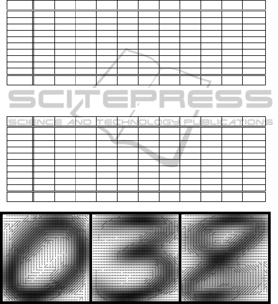
Table 3: Classification error matrix obtained by means of multivariate Bernoulli mixtures (the total number of components
M=1571, number of parameters: 1462373). The last column contains the percentage of false negative decisions. The last row
contains the total frequencies of false positive rates in percent of the respective class test patterns with the global error rate in
bold.
CLASS 0 1 2 3 4 5 6 7 8 9 false n.
0 19950 8 43 19 39 32 36 0 38 17 1.1 %
1 2 22162 30 4 35 7 18 56 32 6 0.9 %
2 32 37 19742 43 30 9 8 29 90 16 1.5 %
3 20 17 62 20021 4 137 2 28 210 55 2.6 %
4 11 6 19 1 19170 11 31 51 30 247 2.1 %
5 25 11 9 154 4 17925 39 6 96 34 2.1 %
6 63 10 17 6 23 140 19652 1 54 3 1.6 %
7 7 12 73 10 73 4 0 20497 22 249 2.1 %
8 22 25 53 97 30 100 11 11 19369 72 2.1 %
9 15 13 25 62 114 22 3 146 93 19274 2.5 %
false p. 0.9% 0.7% 2.7% 2.0% 1.7% 2.3% 0.7% 1.6% 3.3% 3.5% 1.84%
Table 4: Classification error matrix obtained by means of dependence-tree mixtures (number of components M=400, number
of parameters: 819200). The last column contains percentage of false negative decisions. The last row contains false positive
rates in percent of the respective class test patterns with the global error rate in bold.
CLASS 0 1 2 3 4 5 6 7 8 9 false n.
0 19979 11 62 21 18 26 25 2 28 10 1.0 %
1 5 21981 78 13 74 1 20 155 21 4 1.7 %
2 22 15 19777 72 26 5 6 35 72 6 1.3 %
3 20 10 66 20169 1 120 1 20 122 27 1.9 %
4 12 16 13 4 19245 1 13 52 44 177 1.7 %
5 25 5 15 157 8 17874 45 9 129 36 2.3 %
6 100 19 38 25 43 90 19575 1 75 3 2.0 %
7 17 33 108 24 71 0 0 20367 28 299 2.8 %
8 18 30 47 167 27 55 22 17 19337 70 2.3 %
9 12 20 62 74 89 33 3 144 134 19196 2.9 %
false p. 1.4% 0.7% 2.4% 2.7% 1.8% 1.8% 0.7% 1.6% 3.1% 3.2% 1.97%
Figure 1: Mixture of dependence trees for binary data - examples of marginal component probabilities in raster arrangement.
The superimposed optimal dependence structure (defined by maximum-weight spanning tree) reflects the way the respective
numerals have been written.
frequencies of false negative and false positive deci-
sions are also comparable.
Roughly speaking, the dependence-tree mixtures
achieve only slightly better recognition accuracy with
PatternRecognitionbyProbabilisticNeuralNetworks-MixturesofProductComponentsversusMixturesofDependence
Trees
71
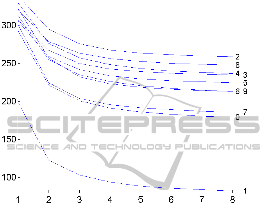
Figure 2: The decreasing information contribution of the dependence structure to the estimated dependence-tree mixtures (the
first eight iterations of the ten estimated class-conditional distributions). The EM algorithm tends to suppress the information
contribution of the dependence structures to the optimal estimate.
a comparable number of parameters, but the most
complex model (M=500) already seems to overfit.
Expectedly, the dependence tree mixtures needed
much less components for the best performance but
they have stronger tendency to overfitting. The best
recognition accuracy in Table 1 (cf. col. IX) well il-
lustrates the power of the subspace product mixtures.
The most surprising result of the numerical exper-
iments is the decreasing importance of the component
dependence structure during the EM estimation pro-
cess. We have noticed that the cumulative weight of
all dependence trees expressed by the weighted sum
Σ
′
=
∑
m∈M
w
′
m
N
∑
n=2
I ( f
′
n|m
, f
′
k
n
|m
)} (34)
is decreasing in the course of EM iterations (cf.
Fig.2). In other words the optimal estimate of the de-
pendence tree mixture tends to suppress the informa-
tion contributionof the dependence structures in com-
ponents, i.e. the component dependence trees tend to
degenerate to simple products. Nevertheless, this ob-
servation is probably typical only for mixtures having
a large number of components since a single product
component is clearly more restrictive than a single de-
pendence tree.
6 CONCLUSIONS
We compare the computational properties of mixtures
of product components and mixtures of dependence
trees in application to recognition of numerals from
the NIST Special Database 19. The underlying clas-
sification problem involves separation of 45 pairs of
classes and therefore the related classification errors
should reveal even small differences between the two
considered classifiers. For the sake of comparison we
have used for each of the considered mixture models
the best solution obtained in series of experiments.
NCTA2014-InternationalConferenceonNeuralComputationTheoryandApplications
72

The detailed description of the classification perfor-
mance (cf. Table 3, Table 4) shows that the recog-
nition accuracy of both models is comparable. It
appears that, in our case, the dependence structure
of components does not improve the approximation
power of the product mixture essentially and, more-
over, the information contribution of the dependence
structure decreases in the course of EM iterations as
shown in Fig. 2. Thus, the optimal estimate of the
dependence tree mixture tends to approach a simple
product mixture model. However, this observation is
probably related to the large number of components
only.
We assume that the dependence tree distribution
is advantageous if we try to fit a small number of
components to a complex data set. However, in case
of a large number of multidimensional components
the component functions are almost non-overlapping
(Grim and Hora, 2010), the structural parameters tend
to fit to small compact subsets of data and the struc-
turally modified form of the components is less im-
portant. We can summarize the properties of depen-
dence tree mixtures as follows:
In Case of a Large Number of Components:
• intuitively, the large number of components is the
main source of the resulting approximation power
• dependence structure of components does not im-
prove the approximation power of product mix-
tures essentially
• the total information contribution of the com-
ponent dependence structures decreases in the
course of EM iterations
• the optimal estimate of the dependence tree mix-
ture tends to approach a simple product mixture
model
In Case of a Small Number of Components:
• a single dependence tree component is capable
to describe the statistical relations between pairs
variables
• consequently, the approximation power of a single
dependence tree component is much higher than
that of a product component
• information contribution of the dependence struc-
ture can increase in the course of EM iterations
• dependence structure of components can essen-
tially improve the approximation quality
In this sense, the computational properties of depen-
dence tree mixtures provide an additional argument
to prefer the product mixture models in case of large
multidimensional data sets.
From the point of view of neural networks and re-
gardless of the computational aspects, the concept of
dependence tree distribution could help to clarify the
role of dendritic ramification in the highly selective
excitability of neurons. The output of formal neu-
rons is usually defined by thresholding the activation
sum of weighted synaptic inputs. Unlike this formal
summation model assuming statistically independent
inputs the thin dendritic branches of biological neu-
rons may be depolarized by weak signals which can
facilitate the conditional activation of the neuron as
a whole. In other words, it is assumed that easily ex-
citable thin dendritic branches may facilitate the prop-
agation of excitation to neural body. The effect of
facilitation could be modeled by the conditional dis-
tributions of the dependence-tree components.
ACKNOWLEDGEMENTS
This work was supported by the Czech Science Foun-
dation Projects No. 14-02652S and P403/12/1557.
REFERENCES
Boruvka, O. (1926). On a minimal problem, Transaction of
the Moravian Society for Natural Sciences (in czech),
No. 3.
Bouguila, N., Ziou, D. and Vaillancourt, J. (2004). Unsuper-
vised learning of a finite mixture model based on the
Dirichlet distribution and its application. IEEE Trans.
on Image Processing, Vol. 13, No. 11, pp. 1533-1543.
Chow, C. and Liu, C. (1968). Approximating discrete
probability distributions with dependence trees, IEEE
Trans. on Information Theory, Vol. IT-14, No.3, pp.
462- 467.
Dempster, A.P., Laird, N.M. and Rubin, D.B. (1977). Max-
imum likelihood from incomplete data via the EM al-
gorithm. J. Roy. Statist. Soc., B, Vol. 39, pp. l-38.
Day, N.E. (1969). Estimating the components of a mixture
of normal distributions, Biometrika, Vol. 56, pp. 463-
474.
Grim, J. (1982). On numerical evaluation of maximum
- likelihood estimates for finite mixtures of dis-
tributions, Kybernetika, Vol.l8, No.3, pp.173-190.
http://dml.cz/dmlcz/124132
Grim, J. (1984). On structural approximating multivariate
discrete probability distributions, Kybernetika, Vol.
20, No. 1, pp. 1-17. http://dml.cz/dmlcz/125676
Grim, J. (1986). Multivariate statistical pattern recognition
with nonreduced dimensionality, Kybernetika, Vol.
22, No. 2, pp. 142-157. http://dml.cz/dmlcz/125022
Grim, J. (1996). Design of multilayer neural networks by
information preserving transforms. In Third European
Congress on Systems Science. (Eds. Pessa E., Penna
PatternRecognitionbyProbabilisticNeuralNetworks-MixturesofProductComponentsversusMixturesofDependence
Trees
73

M. P., Montesanto A.). (Edizioni Kappa, Roma 1996)
977–982.
Grim, J. (1999). Information approach to structural opti-
mization of probabilistic neural networks, In Proc. 4th
System Science European Congress, Eds. Ferrer, L. et
al., Valencia: Soc. Espanola de Sistemas Generales,
pp. 527-540.
Grim, J. (1999b). A sequential modification of EM al-
gorithm, In Studies in Classification, Data Analysis
and Knowledge Organization, Eds. Gaul W., Locarek-
Junge H., Springer 1999, pp. 163 - 170.
Grim, J. (2006). EM cluster analysis for categorical data, In
Structural, Syntactic and Statistical Pattern Recogni-
tion. Eds. Yeung D. Y., Kwok J. T., Fred A., Springer:
Berlin, LNCS 4109, pp. 640-648.
Grim, J. (2007). Neuromorphic features of probabilistic
neural networks. Kybernetika, Vol. 43, No. 5, pp.697-
712. http://dml.cz/dmlcz/135807
Grim, J. (2014). Sequential pattern recognition by maxi-
mum conditional informativity, Pattern Recognition
Letters, Vol. 45C, pp. 39-45.
http:// dx.doi.org/10.1016/j.patrec.2014.02.024
Grim, J., Haindl, M., Somol, P. and P. Pudil (2006). A sub-
space approach to texture modelling by using Gaus-
sian mixtures, In Proceedings of the 18th IAPR In-
ternational Conference on Pattern Recognition ICPR
2006, Eds. B. Haralick, T.K. Ho, Los Alamitos, IEEE
Computer Society, pp. 235-238.
Grim, J. and Hora, J. (2008). Iterative principles of recog-
nition in probabilistic neural networks, Neural Net-
works. Vol. 21, No. 6, pp. 838-846.
Grim, J. and Hora, J. (2009). Recognition of Properties
by Probabilistic Neural Networks, In Artificial Neu-
ral Networks - ICANN 2009, Springer: Berlin, LNCS
5769, pp. 165-174.
Grim, J. and Hora, J. (2010). Computational Properties
of Probabilistic Neural Networks, In Artificial Neu-
ral Networks - ICANN 2010 Part II, Springer: Berlin,
LNCS 5164, pp. 52-61.
Grim, J., Hora, J., Boˇcek P., Somol, P. and Pudil, P. (2010).
Statistical Model of the 2001 Czech Census for Inter-
active Presentation, Journal of Official Statistics. Vol.
26, No. 4, pp. 673694. http://ro.utia.cas.cz/dem.html
Grim, J., Kittler, J., Pudil, P. and Somol, P. (2002). Multi-
ple classifier fusion in probabilistic neural networks,
Pattern Analysis and Applications, Vol. 5, No. 7, pp.
221-233.
Grim, J., Pudil, P. and Somol, P. (2000). Recognition of
handwritten numerals by structural probabilistic neu-
ral networks, In Proceedings of the Second ICSC Sym-
posium on Neural Computation, Berlin, 2000. (Bothe
H., Rojas R. eds.). ICSC, Wetaskiwin, pp. 528-534.
Grim, J., Pudil, P. and Somol, P. (2002b). Boosting in proba-
bilistic neural networks, In Proceedings of the 16th In-
ternational Conference on Pattern Recognition, (Kas-
turi R., Laurendeau D., Suen C. eds.). IEEE Computer
Society, Los Alamitos, pp. 136–139.
Grim, J., Somol, P., Haindl, M. and Daneˇs, J. (2009).
Computer-Aided Evaluation of Screening Mammo-
grams Based on Local Texture Models, IEEE Trans.
on Image Processing, Vol. 18, No. 4, pp. 765-773.
Hasselblad, V. (1966). Estimation of prameters for a mix-
ture of normal distributions, Technometrics, Vol. 8, pp.
431-444.
Hasselblad, V. (1969). Estimation of finite mixtures of dis-
tributions from the exponential family, Journal of
Amer. Statist. Assoc., Vol. 58, pp. 1459-1471.
Hebb, D.O. (1949). The Organization of Behavior: A Neu-
ropsychological Theory, (New York: Wiley 1949).
Hosmer Jr, D.W. (1973). A comparison of iterative maxi-
mum likelihood estimates of the parameters of a mix-
ture of two normal distributions under three different
types of sample, Biometrics, pp. 761-770.
Kirshner, S. and Smyth, P. (2007). Infinite mixtures of trees,
In Proceedings of the 24th International Conference
on Machine Learning (ICML’07), Ed. Zoubin Ghahra-
mani, ACM, New York, USA, pp. 417-423.
Kruskal, J.B. (1956). On the shortest spanning sub-tree of a
graph, Proc. Amer. Math. Soc., No. 7, pp. 48-50.
Kullback, S. and Leibler, R.A. (1951). On Information and
Sufficiency, The Annals of Mathematical Statistics,
Vol. 22, No. 1, pp. 79-86.
Lowd, D. and Domingos, P. (2005). Naive Bayes models
for probability estimation, In Proceedings of the 22nd
international conference on machine learning, ACM
2005, pp. 529-536.
Markley, S.C. and Miller, D.J. (2010). Joint parsimonious
modeling and model order selection for multivariate
Gaussian mixtures, IEEE Journal of Selected Topics
in Signal Processing, Vol. 4, No. 3, pp. 548-559.
Meila, M. and Jordan, M.I. (1998). Estimating dependency
structure as a hidden variable, In Proceedings of the
1997 Conference on advances in neural information
processing systems 10, pp. 584-590.
Meila, M. and Jaakkola T. (2000). Tractable Bayesian
Learning of Tree Belief Networks, In Proceedings of
the 16th Conference on Uncertainty in Artificial Intel-
ligence, pp. 380-388.
Meila, M. and Jordan, M.I. (2001). Learning with mixtures
of trees, Journal of Machine Learning Research, Vol.
1, No. 9, pp. 1-48.
Prim, R.C. (1957). Shortest connection networks and some
generalizations, Bell System Tech. J., Vol. 36 , pp.
1389-1401.
Schlesinger, M.I. (1968). Relation between learning and
self learning in pattern recognition, (in Russian),
Kibernetika, (Kiev), No. 2, pp. 81-88.
Vajda, I. Theory of statistical inference and information,
Kluwer Academic Publishers (Dordrecht and Boston),
1989.
Wolfe, J.H. (1970). Pattern clustering by multivariate mix-
ture analysis, Multivariate Behavioral Research, Vol.
5, pp. 329-350.
NCTA2014-InternationalConferenceonNeuralComputationTheoryandApplications
74

APPENDIX
Maximum-weight Spanning Tree
The algorithm of Boruvka-Kruskal (cf. (Kruskal,
1956), (Chow and Liu, 1968)) assumes ordering of all
N(N − 1)/2 edge weights in descending order. The
maximum-weight spanning tree is then constructed
sequentially, starting with the first two (heaviest)
edges. The next edges are added sequentially in de-
scending order if they do not form a cycle with the
previously chosen edges. Multiple solutions are pos-
sible if several edge weights are equal, but they are
ignored as having the same maximum weight.
The algorithm of Prim (Prim, 1957) does not need
any ordering of edge weights. We start from any
variable by choosing the neighbor with the maximum
edge weight. This first edge of the maximum-weight
spanning tree is then sequentially extended by adding
the maximum-weight neighbors of the currently cho-
sen subtree. Again, any ties may be decided arbitrar-
ily since we are not interested in multiple solutions.
Both Kruskal and Prim refer to an “obscure Czech
paper” of Otakar Boruvka from the year 1926 giving
an alternative construction of the minimum-weight
spanning tree and the corresponding proof of unique-
ness (Boruvka, 1926). The algorithm of Prim can be
summarized as follows (in C-pseudo-code).
It can be seen that in case of dependence-tree mix-
tures with many components the application of the
algorithm of Kruskal (cf. (Kruskal, 1956)) may be-
come prohibitive in high-dimensional spaces because
the repeated ordering of the edge-weights for all com-
ponents is time-consuming (cf. (Meila and Jordan,
1998, 2001; Meila and Jaakkola, 2000)).
//**********************************************
// Maximum-weight spanning tree construction
//**********************************************
//
// NN........ number of nodes, N=1,2,...,NN
// T[N]...... characteristic function of the
// defined part of spanning tree
// E[N][K]... positive weight of the edge <N,K>
// A[K]...... index of the heaviest neighbor
// of node K in the defined subtree
// GE[K]..... greatest edge weight between the
// node K and the defined subtree
// K0........ index of the most heavy neighbor
// of the defined part of tree
// SUM....... total weight of the spanning tree
// spanning tree: {<2,A[2]>,...,<NN,A[NN]>}
//**********************************************
for(N=1; N<=NN; N++) // initial values
{
GE[N]=-1; T[N]=0; A[N]=0;
} // end of N-loop
N0=1; T[N0]=1; K0=0;
//*****************************************
for(I=2; I<=NN; I++) // spanning tree loop
{
FMAX=-1E0;
for(N=2; N<=NN; N++)
if(T[N]<1)
{
F=E[N0][N];
if(F>GE[N]) {GE[N]=F; A[N]=N0;
}
else F=GE[N];
if(F>FMAX) {FMAX=F; K0=N;}
} // end of N-loop
N0=K0; T[N0]=1;
SUM+=FMAX;
} // end of I-loop
//**********************************************
// end of spanning tree construction
//**********************************************
PatternRecognitionbyProbabilisticNeuralNetworks-MixturesofProductComponentsversusMixturesofDependence
Trees
75
