Derivative Free Training of Recurrent Neural Networks
A Comparison of Algorithms and Architectures
Branimir Todorović
1,4
, Miomir Stanković
2,4
and Claudio Moraga
3,4
1
Faculty of Natural Sciences and Mathematics, University of Niš, Niš, Serbia
2
Faculty of Occupational Safety, University of Niš, Niš, Serbia
3
European Centre for Soft Computing, 33600 Mieres, Spain
4
Technical University of Dortmund, 44221 Dortmund, Germany
Keywords: Recurrent Neural Networks, Bayesian Estimation, Nonlinear Derivative Free Estimation, Chaotic Time
Series Prediction.
Abstract: The problem of recurrent neural network training is considered here as an approximate joint Bayesian
estimation of the neuron outputs and unknown synaptic weights. We have implemented recursive estimators
using nonlinear derivative free approximation of neural network dynamics. The computational efficiency
and performances of proposed algorithms as training algorithms for different recurrent neural network
architectures are compared on the problem of long term, chaotic time series prediction.
1 INTRODUCTION
In this paper we consider the training of Recurrent
Neural Networks (RNNs) as derivative free
approximate Bayesian estimation. RNNs form a
wide class of neural networks with feedback
connections among processing units (artificial
neurons). Neural networks with feed forward
connections implement static input-output mapping,
while recurrent networks implement the mapping of
both input and internal state (represented by outputs
of recurrent neurons) into the future internal state.
In general, RNNs can be classified as locally
recurrent, where feedback connections exist only
from a processing unit to itself, and globally
recurrent, where feedback connections exist among
distinct processing units. The modeling capabilities
of globally recurrent neural networks are much
richer than that of the simple locally recurrent
networks.
There exist a group of algorithms for training
synaptic weights of recurrent neural networks that
are based on the exact or approximate computation
of the gradient of an error measure in the weight
space. Well known approaches that use methods for
exact gradient computation are back-propagation
through time (BPTT) and real time recurrent
learning (RTRL) (Williams and Zipser, 1989;
Williams and Zipser, 1990). Since BPTT and RTRL
are using only first-order derivative information,
they exhibit slow convergence. In order to improve
the speed of the RNN training, a technique known as
teacher forcing has been introduced (Williams and
Zipser, 1989). The idea is to use the desired outputs
of the neurons instead of the obtained to compute the
future outputs. In this way the training algorithm is
focused on the current time step, given that the
performance is correct on all earlier time steps.
However, in its basic form teacher forcing is not
always applicable. It clearly cannot be applied in
networks where feedback connections exist only
from hidden units, for which the target outputs are
not explicitly given. The second important case is
the training on noisy data, where the target outputs
are corrupted by noise. Therefore, to apply teacher
forcing in such cases, a true target outputs of
neurons have to be estimated somehow.
The well-known extended Kalman filter
(Anderson and Moore, 1979), as a second order
sequential training algorithm and state estimator
offers the solution to the both stated problems. It
improves the learning rate by exploiting second
order information on criterion function and
generalizes the teacher forcing technique by
estimating the true outputs of the neurons.
The extended Kalman filter can be considered as
the approximate solution of the recursive Bayesian
state estimation problem. The problem of estimating
the hidden state of a dynamic system using
observations which arrive sequentially in time is
76
Todorovi
´
c B., Stankovi
´
c M. and Moraga C..
Derivative Free Training of Recurrent Neural Networks - A Comparison of Algorithms and Architectures.
DOI: 10.5220/0005081900760084
In Proceedings of the International Conference on Neural Computation Theory and Applications (NCTA-2014), pages 76-84
ISBN: 978-989-758-054-3
Copyright
c
 2014 SCITEPRESS (Science and Technology Publications, Lda.)

very important in many fields of science,
engineering and finance. The hidden state of some
dynamic system is represented as a random vector
variable, and its evolution in time
,...}2,1,{ kx
k
is
described by a so called dynamic or process
equation:
),,(
1 kkkkk
duxfx

 ,
(1)
where
xdx
nnn
k
RRf 

: is nonlinear function,
and
,...}2,1,{ kd
k
is an i.i.d. process noise
sequence, while
x
n and
d
n are dimensions of the
state and process noise vectors respectively. The
hidden state is known only through the measurement
(observation) equation:
),(
kkkk
vxhy  ,
(2)
where
y
vx
n
nn
k
RRh 

: is nonlinear function,
and
,...}2,1,{ kv
k
is an i.i.d. measurement noise
sequence, and
y
n
and
v
n are dimensions of the
measurement and measurement noise vectors,
respectively.
In a sequential or recursive Bayesian estimation
framework, the state filtering probability density
function (pdf)
)(
:0 kk
yxp , (where
k
y
:0
denotes the
set of all observations
},...,,{
10:0 kk
yyyy

up to the
time step k), represents the complete solution. The
optimal state estimate with respect to any criterion
can be calculated based on this pdf.
The recursive Bayesian estimation algorithm
consists of two steps: prediction and update. In the
prediction step the previous posterior
)(
1:01  kk
yxp is projected forward in time, using
the probabilistic process model:
kkkkkkk
dxyxpxxpyxp )()()(
1:0111:0 

 ,
(3)
where the state transition density function
)(
1kk
xxp is completely specified by )(

f and the
process noise distribution
)(
k
dp .
In the second step, the predictive density is
updated by incorporating the latest noisy
measurement
k
y using the observation likelihood
)(
kk
xyp to generate the posterior:




kkkkk
kkkk
kk
dxyxpxyp
yxpxyp
yxp
)()(
)()(
)(
1:0
1:0
:0
(4)
This recursive estimation algorithm can be
applied to RNN training after representing the time
evolution of neurons outputs and connection
weights, as well as their observations, in the form of
the state space model. The hidden state of the
recurrent neural network
k
x is a stacked vector of
recurrent neurons outputs
k
s and connection
weights
k
w . Its evolution in time can be represented
by the following dynamic equation.


















k
k
wk
skkk
k
k
dw
dwusf
w
s
1
11
),,,(
,
(5)
where
k
s
d
and
k
w
d
represent dynamic noise
vectors.
The outputs of the neurons are obtained through
the following observation equation:
),,(
kkkk
vwshy

.
(6)
The recurrence relations (3) and (4) are only
conceptual solutions and the posterior density
)(
:0 kk
yxp cannot be determined analytically in
general. The restrictive set of cases includes the well
known Kalman filter, which represents the optimal
solution of (3) and (4) if the prior state density
)()(
000
xpyxp

, the process noise as well as the
observation noise densities are Gaussians, and
)(

f
and
)(

h are linear functions.
In case of RNN training,
)(f and )(

h are
nonlinear in general and an analytic solution is not
tractable, therefore some approximations and
suboptimal solutions have to be considered. The
well known suboptimal solution is the Extended
Kalman Filter (EKF), which assumes the Gaussian
property of noise and uses the Taylor expansion of
)(

f and )(

h (usually up to the linear term) to
obtain the recursive estimation for
)(
:0 kk
yxp . The
EKF has been successfully applied in RNN training
(Todorović et al., 2003; Todorović et al., 2004) due
to important advantages compared to RTRL and
BPTT: faster convergence and generalization of
teacher forcing. Recently, families of new derivative
free filters have been proposed as an alternative to
EKF for estimation in nonlinear systems. Divided
Difference Filters (DDF), derived in (Nørgaard et
al., 2000), are based on polynomial approximation
of nonlinear transformations using a
multidimensional extension of Stirling’s
interpolation formula. The Unscented Kalman Filter
(UKF) (Julier and Uhlmann, 1997) uses the true
nonlinear models and approximates the state
distribution using deterministically chosen sample
points. Surprisingly, both the DDF and the UKF
result in similar equations and are usually called
DerivativeFreeTrainingofRecurrentNeuralNetworks-AComparisonofAlgorithmsandArchitectures
77

derivative free filters (Van der Merwe and Wan,
2001).
The rest of the paper is organized as follows. In
the second section recursive Bayesian estimator is
approximated by linear minimum mean square error
estimator (MMSE), which recursively updates only
the first two moments of the relevant probability
densities. The problem that remains to be solved is
propagating these moments through the nonlinear
mapping of the process equation and the observation
equation. In the third section we describe three
approaches to this problem: a linearization of the
nonlinear mapping using a Taylor series expansion,
a derivative free unscented transform and a
derivative free polynomial approximation using a
multidimensional extension of the Stirling’s
interpolation formula. In the fourth section we give
the state space models of three globally recurrent
neural networks: fully connected, Elman and Non-
linear AutoRegresssive with eXogenous inputs
(NARX) recurrent neural networks. We trained them
by applying approximate recursive Bayesian joint
estimation of the recurrent neurons outputs and
synaptic weights. The results of applying three
different estimation algorithms in training three
different architectures of recurrent neural networks
are given in the last section.
2 LINEAR MMSE ESTIMATION
OF THE NONLINEAR STATE
SPACE MODEL
An analytically tractable solution of the problem of
recursive Bayesian estimation framework can be
obtained based on the assumption that the state
estimator
k
x
ˆ
can be represented as a linear function
of the current observation
k
y :
kkkk
byAx


ˆ
,
(7)
where matrix
k
A and vector
k
b are derived by
minimizing mean square estimation error criterion:
0: 1
ˆˆ
()()(, )
T
kkkkkkkkkk
R
x x x x p x y y dx dy

 

.
(8)
Note that the condition
0


kk
bR is
equivalent to the requirement that the estimator is
unbiased:
0),()(
1:0


 kkkkkkkkk
dydxyyxpbyAx
,
(9)
from which we obtain,


kkkk
yAxb
ˆˆ
, )
ˆ
(
ˆˆ


kkkkk
yyAxx ,
(10)
where




kkkkkkk
dxyxpxyxEx )(][
ˆ
1:01:0
and




kkkkkkk
dyyypyyyEy )(][
ˆ
1:01:0
.
Both the condition
0
kk
AR and the
unbiasedness of the estimator result in the well
known orthogonality principle, which states that the
estimation error is orthogonal to the current
observation, and, consequently:
0),(
)
ˆ
))(
ˆ
(
ˆ
(
1:0





kkkkk
T
kkkkkkk
dydxyyxp
yyyyAxx
.
(11)
From (11) we obtain the matrix
1

kkk
yyxk
PPA ,
where
])
ˆ
)(
ˆ
([
1:0 


k
T
kkkky
yyyyyEP
k
(12b)
])
ˆ
)(
ˆ
([
1:0 


k
T
kkkkyx
yyyxxEP
kk
(12c)
Note that
k
y
P
must be invertible, that is
measurements
k
y have to be linearly independent.
Finally, after replacing
1

kkk
yyxk
PPA we obtain
the linear MMSE estimator:
)
ˆ
(
ˆˆ
1 

kkyyxkk
yyPPxx
kkk
.
(13a)
The matrix Mean Square Error (MSE)
corresponding to (13):
T
yxyyxx
T
kkkk
kkkkkk
PPPPxxxxE
1
])
ˆ
)(
ˆ
[(


.
(13b)
is used as the approximation of the estimator
covariance
])
ˆ
)(
ˆ
[(
T
kkkkx
xxxxEP
k
 .
If the dynamic and the observation models are
linear and process and observation noises are
Gaussian, the linear MMSE estimator is the best
MMSE estimator and is equal to the conditional
mean
]/[
:0 kk
yxE , otherwise it is the best within the
class of linear estimators.
The problem that remains to be solved is the
estimation of the statics of a random variable
propagated trough the nonlinear transformation.
kkk
kkkkkk
dddxdp
yxpduxfx
1
1:011
)(
)(),,(
ˆ





(14a)
kkkkk
T
kkkkkkkkx
dvdxdpyxp
xduxfxduxfP
k
11:01
11
)()(
)
ˆ
),,(()
ˆ
),,((








(14b)




kkkkkkkkk
dvdxvpyxpvuxhy )()(),,(
ˆ
1:0
(14c)
kkkkk
T
kkkkkkkky
dvdxvpyxp
yvuxhyvuxhP
k
)()(
)
ˆ
),,()(
ˆ
),,((
1:0 




(14d)
NCTA2014-InternationalConferenceonNeuralComputationTheoryandApplications
78

kkkkk
T
kkkkkkyx
dvdxvpyxp
yvuxhxxP
kk
)()(
)
ˆ
),,()(
ˆ
(
1:0 




(14e)
The problem can be considered in a general.
Suppose that x is a random variable with mean
x
ˆ
and covariance
x
P . A random variable y is related
to x through the nonlinear function
)(xfy  . We
wish to calculate the mean
y
ˆ
and the covariance
y
P
of y.
2.1 Extended Kalman Filter
The extended Kalman filter is based on the
multidimensional Taylor series expansion of
)(xf .
We shall consider only the first order EKF, obtained
by excluding the nonlinear terms of Taylor series
expansion:
xxfxfxxfxf
x


 )
ˆ
()
ˆ
()
ˆ
()(
(15)
where
xx
x
xfxf
ˆ
)
ˆ
(



is the Jacobian of the
nonlinear function and
x is a zero mean random
variable with covariance
x
P .
In this way the prediction of the state is given by:
kkkk
duxfx 


),
ˆ
(
ˆ
1
(16a)
T
kkk
T
kxkx
GQGFPFP
kk



1
(16b)
where
fF
k
x
k
1
ˆ


, fG
k
d
k
 , ][
kk
dEd  ,
][
T
kkk
ddEQ 
.
The prediction of the observation is given by:
kkk
vxhx 

)
ˆ
(
ˆ
(17a)
T
kkk
T
kxky
LRLHPHP
kk


(17b)
where
hH
k
x
k


ˆ
,
hL
k
vk

,
][
kk
vEv 
,
and
][
T
kkk
vvER 
.
2.2 Divided Difference Filter
In (Nørgaard et al., 2000) Nørgaard et al. proposed a
new set of estimators based on a derivative free
polynomial approximation of nonlinear
transformations using a multidimensional extension
of Stirling’s interpolation formula. This formula is
particularly simple if only the first and second order
polynomial approximation is considered:
fDfDxfxf
xx
2
~~
)
ˆ
()(


(18)
where divided difference operators are defined by:
)(
1
~
1
xfx
h
fD
n
p
pppx













(19)
p

is a “partial” difference operator:
)5.0()5.0
ˆ
()
ˆ
(
ppp
ehxfehxfxf  
(20)
and
p

is an average operator:
))5.0
ˆ
()5.0
ˆ
((5.0)
ˆ
(
ppp
ehxfehxfxf 






(21)
where
p
e is the p-th unit vector.
Applying a stochastic decoupling of the variables
in x by the following transformation xSz
x
1
 , (
x
S
is the Cholesky factor of the covariance matrix
T
xxx
SSP  ), an approximation of the mean and the
covariance of
)(xfy

is obtained:
))()((
2
1
)(
ˆ
1
,,
22
2





n
p
pxpx
hsxfhsxf
h
xf
h
nh
y
(22a)
T
,,
1
,,
4
2
T
,,
1
,,
2
))
ˆ
(2)
ˆ
()
ˆ
((
))
ˆ
(2)
ˆ
()
ˆ
((
4
1
))
ˆ
()
ˆ
((
))
ˆ
()
ˆ
((
4
1
xfhsxfhsxf
xfhsxfhsxf
h
h
hsxfhsxf
hsxfhsxf
h
P
pxpx
n
p
pxpx
pxpx
n
p
pxpxy










(22b)
Nørgaard et al. have derived the alternative
covariance estimate as well (Nørgaard et al., 2000):
T
2
2
1
T
,,
2
1
T
,,
2
)
ˆ
)
ˆ
()
ˆ
)
ˆ
((
)
ˆ
)
ˆ
()
ˆ
)
ˆ
((
2
1
)
ˆ
)
ˆ
()
ˆ
)
ˆ
((
2
1
yxfyxf
h
nh
yhsxfyhsxf
h
yhsxfyhsxf
h
P
n
p
pxpx
n
p
pxpxy









(23)
This estimate is less accurate than (22b).
Moreover, for
nh 
2
the last term becomes
negative semi-definite with a possible implication
that the covariance estimate (23) becomes non-
positive definite too. The reason why this estimate is
considered here is to provide a comparison with the
covariance estimate obtained by the Unscented
Transformation described in the next subsection.
2.3 Unscented Kalman Filter
Julier and Uhlman proposed the Unscented
Transformation (UT) (Julier and Uhlmann, 1997) in
order to calculate the statistics of a random variable
x
propagated through the nonlinear function
)(xfy

. The
x
n -dimensional continuous random
DerivativeFreeTrainingofRecurrentNeuralNetworks-AComparisonofAlgorithmsandArchitectures
79

variable
x
with mean x
ˆ
and covariance
x
P is
approximated by
12 
x
n sigma points
p
X with
corresponding weights
p

,
x
np 2,...,1,0 :
xx
nnnx  )(,)(,
ˆ
2
0

0
X fo
r
np ...,2,1
)(5.0
ˆ
,
  nsnx
ppxp
X
)(5.0
ˆ
,
 

nsnx
xx
nppxnp
X
where

determines the spread of the sigma points
around
x
ˆ
(usually 14.1 



e ) and



is the
scaling parameter, usually set to 0 or
x
n3 (Julier
and Uhlmann, 1997).
px
s
,
is the p-th row or column
of the matrix square root of
x
P .
Each sigma point is instantiated through the
function
)(f to yield the set of transformed sigma
points
)(
0
XY f
i

, and the mean y
ˆ
of the
transformed distribution is estimated by:
))
ˆ
(
)
ˆ
((
)(2
1
)
ˆ
(
ˆ
,
1
,
2
0
ix
n
i
ix
n
p
pp
snxf
snxf
n
xf
n
y
x













Y
(24)
The covariance estimate obtained by the
unscented transformation is:















n
p
pxpx
n
p
pxpx
n
p
pppy
ysnxfysnxf
n
ysnxfysnxf
n
yxfyxf
n
yyP
x
1
T
,,
1
T
,,
T
2
0
T
)
ˆ
)
ˆ
()
ˆ
)
ˆ
((
)(2
1
)
ˆ
)
ˆ
()
ˆ
)
ˆ
((
)(2
1
)
ˆ
)
ˆ
()
ˆ
)
ˆ
(()
ˆ
)
ˆ







YY ((
(25)
It can be easily verified that for
  nh , the
estimates of the mean (22a) and the covariance (23)
obtained by DDF are equivalent to the estimates (24)
and (25) obtained by UKF. The interval length
h is
set equal to the kurtosis of the prior random variable
x
. For Gaussians it holds 3
2
h .
3 STATE SPACE MODELS OF
GLOBALLY RECURRENT
NEURAL NETWORKS
In order to apply approximate Bayesian estimators
as training algorithm of recurrent neural networks
we need to represent dynamics of RNN in a form of
state space model. In this section we define the state
space models of three representative architectures of
globally recurrent neural networks: Elman, fully
connected, and NARX recurrent neural network.
3.1 Elman Network State Space Model
In Elman RNNs adaptive feedbacks are provided
between every pair of hidden units. The network is
illustrated in Fig.1.a), and the state space model of
the Elman network is given by equations





































H
k
O
k
H
k
w
w
x
H
k
O
k
k
H
k
H
k
H
k
O
k
H
k
d
d
d
w
w
uwxf
w
w
x
1
1
11
),,(
(26a)
),(,
O
k
H
k
O
kk
O
kk
wxhxvxy 
(26b)
where
H
k
x
represents the output of the hidden
neurons in the k-th time step,
O
k
x is the output of
the neurons in the last layer,
O
k
w
1
is the vector of
synaptic weights between the hidden and the output
layer and
H
k
w
1
is the vector of recurrent adaptive
connection weights. Note that in the original
formulation of Elman, these weights were fixed.
Random variables
H
k
x
d ,
O
k
w
d ,
H
k
w
d represent the
process noises.
It is assumed that the output of the network
),(
O
k
H
k
O
k
wxhx  is corrupted by the observation
noise
k
v .
x
x
x
H
O
O
H
H
H
H
H
x
x
1,k
1,k
2,k
n ,k
n ,k
H
u
k
z
-1
z
-1
z
-1
x
x
x
1,k-1
2,k-1
n ,k-1
H
O
y
y
1,k
n ,k
u
k
H
H
H
H
O
O
O
O
z
-1
z
-1
z
-1
z
-1
x
1, -1k
x
1,k
x
1, -1k
x
1,k
x
n , -1k
H
x
n ,k
H
x
x
n , -1k
n ,k
O
O
O
a) Elman b) Fully connected
Figure 1: Elman and fully connected RNN.
3.2 Fully Connected Recurrent
Network State Space Model
In fully connected RNNs adaptive feedbacks are
provided between each pair of processing units
(hidden and output). The state vector of a fully
connected RNN consists of outputs (activities) of
NCTA2014-InternationalConferenceonNeuralComputationTheoryandApplications
80

hidden
H
k
x
and output neurons
O
k
x
, and their
synaptic weights
H
k
w and
O
k
w . The activation
functions of the hidden and thee output neurons are
),,,(
1 k
H
k
H
k
O
k
H
uwxxf

and ),,,(
1 k
O
k
H
k
O
k
O
uwxxf

,
respectively. The network structure is illustrated in
Fig. 1.b).
The state space model of the network is given
by:
















































H
k
O
k
H
k
O
k
w
w
x
x
H
k
O
k
k
H
k
H
k
O
k
H
k
O
k
H
k
O
k
O
H
k
O
k
H
k
O
k
d
d
d
d
w
w
uwxxf
uwxxf
w
w
x
x
1
1
1
1
),,,(
),,,(
(27a)
]0[,
)(
OSOOO
nnnnnk
H
k
O
k
H
k
O
k
k
IHv
w
w
x
x
Hy

















(27b)
The dynamic equation describes the evolution of
neuron outputs and synaptic weights. In the
observation equation, the matrix H selects the
activities of output neurons as the only visible part
of the state vector, where
S
n is the number of
hidden states which are estimated:

HOS
nnn
HO
WW
nn  ,
O
n and
H
n are the
numbers of output and hidden neurons respectively,
O
W
n is the number of adaptive weights of the
output neurons,
H
W
n is the number of adaptive
weights of the hidden neurons.
3.3 NARX Recurrent Neural Network
State Space Model
The non-linear AutoRegressive with eXogenous
inputs (NARX) recurrent neural network usually
outperforms the classical recurrent neural networks,
like Elman or fully connected RNN, in tasks that
involve long term dependencies for which the
desired output depends on inputs presented at times
far in the past.
x
k
O
OO
z
-1
z
-1
z
-1
z
-1
u
u
x
k-1
u
k-1
k
x
k-
u
x
k- 
Figure 2: NARX recurrent neural network.
Here we define the state space model of a NARX
RNN. Adaptive feedbacks are provided between the
output and the hidden units. These feedback
connection and possible input connections are
implemented as FIR filters. The state vector consists
of outputs of the network in
x
 time steps
O
k
x ,
O
k
x
1
,...,
O
k
x
x
1
, the output
O
k
w , and hidden
synaptic
H
k
w weights.





































































H
k
O
k
O
k
x
ux
x
w
w
x
H
k
O
k
O
k
O
k
kkk
O
k
O
k
H
k
O
k
O
k
O
k
O
k
d
d
d
w
w
x
x
wuuxxf
w
w
x
x
x
0
0
),,..,,,..,(
1
1
1
1
111
1
1



(28)
The dynamic equation describes the evolution of
network outputs and synaptic weights.
]0[,
)(
1
1
OSOOO
x
nnnnnk
H
k
O
k
O
k
O
k
O
k
k
IHv
w
w
x
x
x
Hy


























(29)
As in previous examples,
O
n represents the
number of output neurons.
S
n is the number of
hidden states of the NARX RNN:
HO
WW
OS
nnnn



,
O
W
n
is the number of
adaptive weights of output neurons,
H
W
n
is number
of adaptive weights of hidden neurons.
All considered models have nonlinear hidden
neurons and linear output neurons. Two types of
nonlinear activation functions have been used in the
following tests: the sigmoidal and the Gaussian
radial basis function.
4 EXAMPLES
In this section we compare derived algorithms for
sequential training of RNN.
We have evaluated the performance of
algorithms in training three different architectures of
globally recurrent neural networks: fully connected
RNN, Elman RNN with adaptive recurrent
connections and NARX recurrent neural network.
The problem at hand was the long term prediction of
chaotic time series. Implementation of Divided
Difference Filter and Unscented Kalman filter did
DerivativeFreeTrainingofRecurrentNeuralNetworks-AComparisonofAlgorithmsandArchitectures
81

not required linearization of the RNN state space
models. However, in order to apply Extended
Kalman Filter we had to linearize the RNNs state
space models that are to calculate Jacobian of the
RNN outputs with respect to the inputs and synaptic
weights. Note that we did not apply back
propagation through time but standard back
propagation algorithm to calculate the Jacobian. This
was possible because of the joint estimation of RNN
outputs and synaptic weights.
In the process of the evaluation, recurrent neural
networks were trained sequentially on the certain
number of samples. After that they were iterated for
a number of samples, by feeding back just the
predicted outputs as the new inputs of the recurrent
neurons. Time series of iterated predictions were
compared with the test parts of the original time
series by calculating the Normalized Root Mean
Squared Error (NRMSE):




N
k
kk
N
yyNRMSE
1
2
1
)
ˆ
(
2

(30)
where

is the standard deviation of chaotic time
series,
k
y is the true value of sample at time step k ,
and

k
y
ˆ
is the RNN prediction.
Mean and variance of the NRMSE obtained on
30 independent runs, average time needed for
training and number of hidden neurons and adaptive
synaptic weights are given in tables for comparison.
The variance of the process noise
ks
d
,
and
kw
d
,
were exponentially decayed form 1.e-1 and 1.e-3 to
1.e-10, and the variance of the observation noise
k
v
was also exponentially decayed from 1.e-1 to 1.e-10
during the sequential training.
4.1 Mackey Glass Chaotic Time Series
Prediction
In our first example we have considered the long
term iterated prediction of the Mackey Glass time
series. We have applied Divided Difference Filter,
Unscented Kalman Filter and Extended Kalman
Filter for joint estimation of synaptic weights and
neuron outputs of three different RNN architectures:
Elman, fully connected and non-linear
AutoRegressive with eXogenous inputs (NARX)
recurrent neural network.
After sequential adaptation on 2000 samples, a
long term iterated prediction of the next
100

N
samples is used to calculate the NRMSE.
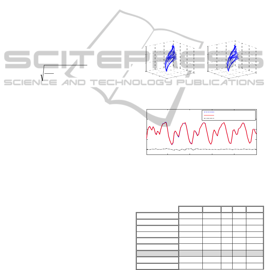
Table 1. contains mean and variance of NRMSE
obtained after 30 independent trials of each
estimator applied on each architecture. We also give
the number of hidden units, the number of adaptable
parameters and time needed for training on 2000
samples. Given these results we can conclude that
the NARX network is superior in both NRMSE of
long term prediction and time needed for training,
compared to other two architectures. As for the
approximate Bayesian estimators, although slightly
slower in our implementation, derivative free filters
(DDF and UKF) are consistently better than EKF,
that is they produced RNN’s with significantly lower
NRMSE.
Sample results of long term prediction using
NARX network with sigmoidal neurons, trained
using DDF are shown in Fig. 3.
0
0.5
1
1.5
0
0.5
1
1.5
0
0.5
1
1.5
x(k-1)
Mackey Glass attractor
x(k-2)
x(k)
0
0.5
1
1.5
0
0.5
1
1.5
0
0.5
1
1.5
x(k-1)
NARX RMLP attractor
x(k-2)
x(k)
a) Phase plot of
k
x versus
1k
x and
2k
x for the
Mackey Glass time series and the NARX RMLP iterated
prediction
2020 2040 2060 2080 2100
0
0.5
1
1.5
2
Time step: k
Chaotic time series
Prediction
Error
b) Comparison of the original chaotic time series and the
NARX RMLP iterated prediction
Figure 3: Mackey Glass chaotic time series prediction.
Table 1: NRMSE of the long term iterated prediction for
various RNN architectures and training algorithms.
Mean Var n
H
n
W
T[s]
DDF_ELMAN_SIG 0.316 8.77e-3 10 121 20.88
UKF_ELMAN_SIG 0.419 3.43e-2 10 121 20.91
EKF_ELMAN_SIG 0.429 5.89e-2 10 121 14.98
DDF_FC_SIG 0.269 7.15e-3 10 131 23.43
UKF_FC_SIG 0.465 8.51e-2 10 131 23.78
EKF_FC_SIG 0.359 8.64e-2 10 131 17.38
DDF_NARX_SIG 0.0874 2.91e-4 5 41 5.64
UKF_NARX_SIG 0.119 1.89e-3 5 41 5.68
EKF_NARX_SIG 0.153 3.37e-3 5 41 4.76
4.2 Hénon Chaotic Time Series
Prediction
In our first example, we consider the prediction of
NCTA2014-InternationalConferenceonNeuralComputationTheoryandApplications
82

the long-term behavior of the chaotic Hénon
dynamics:
2
2
1
3.04.11


kkk
xxx
(31)
RNNs with sigmoidal and Gaussian hidden neurons
(we call this network Recurrent Radial Basis
Function network – RBF network) were trained
sequentially on 3000 samples. After training
networks were iterated for 20 samples by feeding
back the current outputs of the neurons as the new
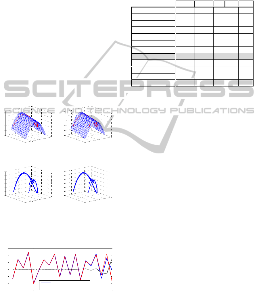
inputs. Figures 4 and 5 show results of prediction
using NARX_RBF network trained by DDF on a
Hénon chaotic time series.
It can be seen from Figures 4.a and 4.b, that,
although the network was trained only using sample
data chaotic attractor, which occupies small part of
the surface defined by equation (31), the recurrent
neural network was able to reconstruct that surface
closely to the original mapping (Fig 4.a), as well as
to reconstruct the original attractor (Fig 4.b).
-2
-1
0
1
2
-2
0
2
-3
-2
-1
0
1
2
x(k-1)
Hénon attractor
x(k-2)
x(k)
-2
-1
0
1
2
-2
0
2
-3
-2
-1
0
1
2
x(k-1)
NARX RRBF attractor
x(k-2)
x(k)
a) Surface plot of the Hénon and NARX_RRBF map; Dots
– chaotic attractor and NARX RRBF attractor
-2
-1
0
1
2
-2
0
2
-1.5
-1
-0.5
0
0.5
1
1.5
x(k-1)
Hénon attractor
x(k-2)
x(k)
-2
-1
0
1
2
-2
0
2
-1.5
-1
-0.5
0
0.5
1
1.5
x(k-1)
NARX RRBF attractor
x(k-2)
x(k)
b) Phase plot of
k
x versus
1k
x and
2k
x for the Hénon
series and NARX RRBF iterated prediction
Figure 4: Hénon chaotic time series prediction: surface
and phase plot.
3000 3005 3010 3015 3020
-1.5
-1
-0.5
0
0.5
1
1.5
Time step: k
Chaotic time series
Prediction
Error
Figure 5: Comparison of the original chaotic time series
and the NARX RRBF iterated prediction.
Results presented in Table 2. show that both DDF
and UKF produce more accurate RNNs than EKF
with comparable training time.
Table 2: Results of long term predictions of the Hénon
chaotic time series.
Mean Var n
H
n
W
T[s]
DDF_ELMAN_SIG 1.73e-2 6.19e-5 4 25 8.34
DDF_ELMAN_RBF 6.02e-2 3.89e-4 3 22 7.76
UKF_ELMAN_SIG 7.29e-2 9.46e-3 4 25 8.53
UKF_ELMAN_RBF 7.24e-2 1.79e-3 3 22 7.91
EKF_ELMAN_SIG 1.69e-1 5.17e-2 4 25 7.69
EKF_ELMAN_RBF 1.01e-1 7.50e-3 3 22 7.96
DDF_NARX_SIG 7.46e-3 3.39e-6 4 17 6.21
DDF_NARX_RBF 4.36e-3 4.15e-6 3 16 5.85
UKF_NARX_SIG 1.28e-2 2.68e-5 4 17 6.37
UKF_NARX_RBF 5.72e-3 7.14e-6 3 16 6.00
EKF_NARX_SIG 1.57e-2 1.65e-5 4 17 5.76
EKF_NARX_RBF 7.07e-3 1.35e-6 3 16 6.17
5 CONCLUSIONS
We considered the problem of recurrent neural
network training as an approximate recursive
Bayesian state estimation. Results in chaotic time
series long term prediction show that derivative free
estimators Divided Difference Filter and Unscented
Kalman Filter considerably outperform Extended
Kalman Filter as RNN learning algorithms with
respect to the accuracy of the obtained network,
while retaining comparable training times.
Experiments also show that of tree considered
architectures: Elman, fully connected and non-linear
AutoRegressive with eXogenous inputs (NARX)
recurrent neural network, NARX is by far superior
in both training time and accuracy of trained
networks in long term prediction.
REFERENCES
Anderson, B. and J. Moore, 1979. Optimal Filtering.
Englewood Cliffs, NJ, Prentice-Hall.
Julier, S. J., and Uhlmann, J. K., A new extension of the
Kalman filter to nonlinear systems. 1997, Proceedings
of AeroSense: The 11
th
international symposium on
aerospace/defence sensing, simulation and controls,
Orlando, FL.
Nørgaard, M., Poulsen, N. K., and Ravn, O., 2000,
Advances in derivative free state estimation for
nonlinear systems, Technical Report, IMM-REP-1998-
15, Department of Mathematical Modelling, DTU.
Todorović, B., Stanković, M., and Moraga, C. 2003, On-
line Learning in Recurrent Neural Networks using
DerivativeFreeTrainingofRecurrentNeuralNetworks-AComparisonofAlgorithmsandArchitectures
83

Nonlinear Kalman Filters. In Proc. of ISSPIT 2003,
Darmstadt, Germany.
Todorović, B., Stanković, M., and Moraga C., 2004,
Nonlinear Bayesian Estimation of Recurrent Neural
Networks. In Proc. of IEEE 4th International
Conference on Intelligent Systems Design and
Applications ISDA 2004, Budapest, Hungary, August
26-28, pp. 855-860.
Van der Merwe, R. and Wan, E. AS. 2001, Efficient
Derivative-Free Kalman Filters for Online Learning.
In Proc. of ESSAN, Bruges, Belgium.
Williams, R. J., & Zipser, D. 1989, A learning algorithm
for continually running fully recurrent neural
networks. Neural Computation, 1, 270-280.
Williams, R. J. and Zipser, D. 1990, Gradient-based
learning algorithms for recurrent connectionist
networks. TR NU_CCS_90-9. Boston, Northeastern
University.
NCTA2014-InternationalConferenceonNeuralComputationTheoryandApplications
84