Speckled Images Segmentation and Algorithm Comparison

Luigi Cinque

, Rossella Cossu

and Rosa Maria Spitaleri

Dipartimento Informatica, Universit´a degli Studi, Sapienza, Via Salaria 113, 00185 Roma, Italy

Istituto per le Applicazioni del Calcolo-CNR, Via dei Taurini 19, 00185 Roma, Italy

Keywords:

Speckle, Image Segmentation, Level Set, Partial Differential Equation.

Abstract:

An image segmentation process, based on the level set method, consists in the time evolution of an initial

curve until it reaches the boundary of the objects to be extracted. Classically the evolution of the initial curve

is determined by a speed function. In this paper, the speed in the level set procedure is characterized by the

combination of two different speed functions and the resulting algorithm is applied to speckled images, like

SAR (Synthetic Aperture Radar) images. In order to assess improvements of the segmentation performance,

the computational process is tested on synthetic and then applied to real images. Performances are evaluated

on synthetic images by using the Hausdorff distance. The real SAR images were acquired during the ERS2

mission.

1 INTRODUCTION

We face the problem of speckled images segmenta-

tion, like the SAR images. It is well known that the

presence of speckle, modeled as a strong multiplica-

tive noise, makes regions detection a very compli-

cated issue.

In the last decades, variational methods, based on

the Γ − convergence property (Mumford and Shah,

1989), (Spitaleri, March and Arena,1999), (Cinque,

Cossu and Spitaleri, 2014) or the level set approach,

(Sethian, 1999), (Sethian, 2001),(Osher and Fedkiw,

2002) (Cinque and Cossu, 2011) leading to solve par-

tial differential equations (PDEs), have been impor-

tant tools for solving image segmentation problems.

References show that we have been developing varia-

tional segmentation algorithms by both approaches.

The level set segmentation is characterized by the

implicit representation of a curve that evolves over

time, deﬁned as the zero level of a 3D level function

(Sethian, 1999), (Sethian, 2001),(Osher and Fedkiw,

2002).

Active contours methods had a fundamental role

in image segmentation. They are computer gener-

ated curves that move within the image to ﬁnd the the

boundaries of the regions under the inﬂuence of inter-

nal and external forces (Kass, Witkin and Terzopulos,

1988) (Chan and Vese, 2001). The evolution of the

curve is carried out in accordance with a speed func-

tion, fundamental step to achieve a good segmenta-

tion.

In this paper we present a new speed, which is the

linear combination of two different speed functions:

the ﬁrst speed, called average-based speed (Ben Ayed,

Mitiche and Belhadj, 2005), (Mitiche and Ben Ayed,

2011) (Ben Salah, Ben Ayed and Mitiche, 2012) de-

pends on the mean gray values of the two regions,

foreground and background, identiﬁed by the curve,

the second speed, called gradient-based speed, de-

pends on the image gradient previously processed

with a SRAD (Speckle Reducing Anisotropic Diffu-

sion) ﬁlter (Yongjian and Acton, 2002) to reduce the

speckle noise.

We compare the results of the segmentation ob-

tained applying the level set equation with the new

combined speed either the average-based or the

gradient-based speed separately. Our approach is val-

idated by tests on synthetic speckled images; in par-

ticular by calculating the Hausdorff distance between

the real contours and computed ones, we compare re-

sults in quantitative way (Huttenlocher, Klanderman

and Rucklidge, 1993).

The Hausdorff distance measures the maximum of

minimum distances between two subsets in a metric

space, in our case between the sets of points belong-

ing to the known and the computed contours of the

test images.

We present and discuss results related to one or more

objects, with non convex boundaries, corrupted by

speckle noise, test images and SAR images. The SAR

PRI (Precision Images)images here segmented were

acquired during ERS2 mission. ERS2 SAR system is

111

Cinque L., Cossu R. and Maria Spitaleri R..

Speckled Images Segmentation and Algorithm Comparison.

DOI: 10.5220/0005166901110118

In Proceedings of the International Conference on Pattern Recognition Applications and Methods (ICPRAM-2015), pages 111-118

ISBN: 978-989-758-077-2

 2015 SCITEPRESS (Science and Technology Publications, Lda.)

capable of 25 m. resolution from an altitude of 800

km, at radar wavelength of 5.7 cm.

The paper is organized as follows. In Section 2,

the level set method is brieﬂy described. In Section

3, speed computation related to level set method is in-

troduced. In Section 4, experimental results, perfor-

mance evaluation on test problems and application to

SAR images are shown. Some conclusions are drawn

in Section 5.

2 MATHEMATICAL MODELING

The level set function is characterized by the implicit

representation of a curve. It is deﬁned as a signed dis-

tance function, where the points of the curve assume

zero value, while at any other point the value of the

function is given by the minimum distance between

this point and the curve.

Since the image segmentation consists in the ex-

tracting the boundary of regions of interest from an

image. This boundary may be considered as a curve

belonging to a family whose time evolution is de-

scribed by a level set equation. In order to resolve this

equation, an iterative process computes the evolution

of the initial curve corresponding to the resolution of

the differential equation in partial derivatives.

2.1 Curve Evolution by Level Set

In order to obtain the governing equation of

a front evolution we consider a family of

parametrized closed contours (t is the parame-

ter) C(x(t),y(t),t) : [0,∞) → R

, generated by

evolving an initial contour C

(x(0),y(0),0). We

underline that in the curves evolution theory the

geometric shape of the contour is determined by the

normal component of the evolution velocity.

If F(x(t),y(t),t) is a scalar function representing

the curve speed in the normal direction~n, the normal

velocity components are

= F(x(t),y(t),t) · n

with ~n ≡ (n

). So that the curve evolves in time

according to the following equation

∂C(x(t),y(t),t)

∂t

= F(x(t),y(t),t) ·~n (1)

Supposing that C(x(t),y(t),t) is a moving front in

the image, if we embed this moving front as the

zero level of a smooth continuous scalar 3D func-

tion φ(x(t),y(t),t), known as the level set func-

tion, the implicit contour at any time t is given by

C(x(t),y(t),t) ≡ {(x(t), y(t))/φ(x(t), y(t),t) = 0}.

By differentiating respect to t the expression

φ(x(t),y(t),t) = 0 the equation of motion for the level

set function may be derived

∂φ(x(t),y(t),t)

∂t

+ F(x(t),y(t),t) · n

∂φ(x(t),y(t),t)

∂x

+ F(x(t),y(t),t) · n

∂φ(x(t),y(t),t)

∂y

= 0

(2)

Being now

∂φ(x(t),y(t),t)

∂x

|∇φ(x(t),y(t),t)|

∂φ(x(t),y(t),t)

∂y

|∇φ(x(t),y(t),t)|

where |∇φ(x(t),y(t),t)| 6= 0 for all (x(t), y(t) ∈

C(x(t),y(t),t), the equation (2) becomes

∂φ(x(t),y(t),t)

∂t

F(x(t),y(t),t)

|∇φ(x(t),y(t),t)|

·[(

∂φ(x(t),y(t),t)

∂x

)

+ (

∂φ(x(t),y(t),t)

∂y

)

] = 0

Moreover for simplicity we can write x ≡ (x(t), y(t)),

C ≡ C(x,y,t)

or also

∂φ(x,t)

∂t

+ F(x,t)|∇φ(x,t)| = 0 (3)

In the following, an important intrinsic geometric

property will be used, that is the curvature of level

set (Sethian, 2001), is given by

k = −∇ ·



∇φ(x,t)

|φ(x,t)|



. (4)

2.2 Level Set Implementation

The numerical implementation of equation (3) is re-

alized by performing a discretization with respect to

time.

In the process of evolution of the curve, the level set

function can lose the properties of the distance for the

sake of approximation. To reduce calculation errors

and ensure stability to the method, the function φ(x,t)

is periodically re-initialized after a certain number of

iterations.

The distance calculation is performed in the pro-

cess of re-initialization, in order to transformthe func-

tion φ(x,t) in a signed distance function (Li, Xu, Gui

and Fox, 2010), by computing the current distance

function.

In the implementation, for the numerical approxima-

tion of the level set equation in a domain Ω ⊂ ℜ

ICPRAM2015-InternationalConferenceonPatternRecognitionApplicationsandMethods

112

we introduce the computational domain Ω

∗

obtained

by considering a uniform partition of Ω in (N − 1) ×

(M − 1) disjoint rectangles Ω

with edges ∆x = ∆y

which usually in an image are ∆x = ∆y = 1.

Let P

i, j

≡ P(x

)(i = 1,...,N; j = 1, ...,M) be a point

in Ω

∗

and φ

i, j

the value of the function φ(x,t) at P

i, j

at time t

The algorithm starts by initializing φ(x,t) as a

signed distance function, depending on interior or ex-

ternal points of curve C

φ(x,t = 0) = ±d

where

d(x) = min

∈C

|x− x

Now, known the value of φ

i, j

, the value φ

n+1

i, j

is com-

puted by a 2-order ENO scheme with the TVD (Total

Variation Diminishing) Runge Kutta scheme for the

time integration. The iterative process ends when the

curve is stable or when it ceases its evolution, that is

at convergence.

We underline that the deﬁnition of φ(x,t) as a

signed distance function is crucial.

Moreover the choice of an appropriate speed function

is a fundamental task for this segmentation approach.

This function is computed by the original image, as it

is described in the following section.

3 CURVE SPEED

In this section we present a synthetic introduction of

the combined speed obtained by the contribution of

the two speed functions (Cinque and Cossu, 2011). In

this work we assume two types of regions, foreground

and background, R

i ∈ {1,2},

Let I(x) be the SAR image intensity which is mod-

eled by a Gamma distribution. After some probabilis-

tic considerations and algebraic manipulations we ob-

tain the average-based speed (Mitiche and Ben Ayed,

2011) in the form

F(x,t) =

= −



logµ

I(x)

− logµ

−

I(x)

+ λk



(5)

where λk is a regularizationterm, with λ ∈ (0,1) and k

the mean curvature function, µ

is the mean intensity,

with a

the area of the region R

, that is

I(x)dx

dx.

The gradient-based function is computed as the gra-

dient magnitude of the original image and represents

the front speed point by point (Cerimele, Cinque and

Cossu, 2009).

It is well known that in images corrupted by strong

noise, the computation of the gradient could detect

false edges. For this reason, the speckle image is pre-

processed by means of the SRAD algorithm which

is an extension of Perona-Malik algorithm (Yongjian

and Acton, 2002), (Perona and Malik, 1990).

The gradient-based speed (Sethian, 1999) is com-

puted on the ﬁltered image

F(x,t) = −

1+ |∇I

′

(x)|

− λk

where I

′

(x) is the image I(x) ﬁltered by SRAD, k is

the curvature and λ ∈ (0,1) is a constant. So, the

speed term is deﬁned in such a way that the curve pro-

ceeds rather fast in low gradient zones, while it wades

through to high gradient ones.

The new velocity is the linear combination of the

average-based and gradient-based speed and it is

given by the following expression:

F(x,t) = −α



log

+ I(x)

− µ



− (1− α)



1+ |∇I

′

(x)|



− λk.

(6)

where α ∈ (0,1) .

We can substitute the speed F(x,t) (6) in the equation

level set (3).

The function φ(x,t) is the computed contour of the

extracted region at the convergence. The segmenta-

tion, indeed, is deﬁned by the convergence for t → ∞

of (3).

The procedure developed by using the combined

speed improves the results obtained by the two speeds

separately. We obtained the best results of segmenta-

tion setting, mainly, the parameter α = 0.5.

4 EXPERIMENTAL RESULTS

In this section we apply the proposed algorithm to

both synthetic and SAR images (Cinque and Cossu,

2011).

4.1 Application to Synthetic Images

We tested the procedure on synthetic images to have

an exact reference of the contours to be detected .

In this paper,to evaluate the efﬁciencyof the proposed

speed, we calculated the Hausdorff distance between

SpeckledImagesSegmentationandAlgorithmComparison

113

the pixels of the known and computed contours of the

synthetic images. Then we show the quantitative and

qualitative comparison between resulting contours.

The Hausdorff distance H measures the maximum of

minimum distances between the points of two con-

tours. Given the contours A = {a

,. .. a

} and B =

,. .. b

}, the Hausdorff distance is deﬁned as

H(A, B) = max(h(A,B),h(B,A))

where

h(A,B) = max

a∈A

min

b∈B

ka− bk

ka− bk is any metric between the points of A

and B (e. g.the Euclidean distance) (Huttenlocher,

Klanderman and Rucklidge, 1993).

The following test image has been synthesized from

an original image without noise, by copying a speckle

pattern from SAR image.

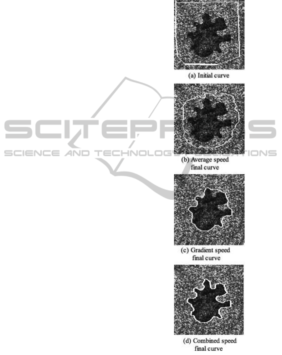
Fig. 1 shows the images with the initial curve (a) and

the corresponding results obtained by applying the

level set equation, using the average-based speed (b),

the gradient-based speed (c) and combined speed (d)

respectively.

As recalled in Section 3, in the case of the compu-

tation of the gradient-based speed, the ﬁlter SRAD

is applied to the image to preserve and enhance the

edges (Yongjian and Acton, 2002). We solve (3) with

(6), varying the parameter α, with α ∈ (0,1) and

setting the parameter λ with λ = 0.3. We recall that

λ ∈ (0,1) and it indicates the weight, associated with

the component speed that depends on the curvature

k. Then the distance H between the known and

computed contours is also computed for performance

evaluation.

The results are the following:

• the chosen initial contour of Fig.1 (a) has the H

distance from the real contour H = 63.78.

• the computed contour of Fig.1 (b), obtained by

setting the parameter α = 0.9, has the H distance

from the real contour H = 43.56. As given by (6),

the value α = 0.9 implies a very low contribution

of the gradient-based speed, thus we can note that

this contour is mainly computed by average-based

speed.

• the computed contour of Fig.1 (c), obtained by

setting the parameter α = 0.1, has the H distance

from the real contour H = 23.02. In this case by

(6), the value α = 0.1 implies the very high contri-

bution of gradient-based speed mainly. As above

written, the level set equation is computed on the

ﬁltered image.

Figure 1: Speckled test image (150×150): (a) Starting con-

tour, (b) ﬁnal contour by average-based speed, (c) ﬁnal con-

tour by gradient-based speed, (d) ﬁnal contour by combined

speed.

ICPRAM2015-InternationalConferenceonPatternRecognitionApplicationsandMethods

114

• the computed contour of Fig. 1 (d), obtained by

setting the parameter α = 0.5, has the H distance

from the known contour H = 3.01. α = 0.5 deter-

mines the best result.

In this type of image the best results are computed, if

the value of alpha is such that the contributions of the

two speeds are similar, that is this α value balances

the results of the two speeds.

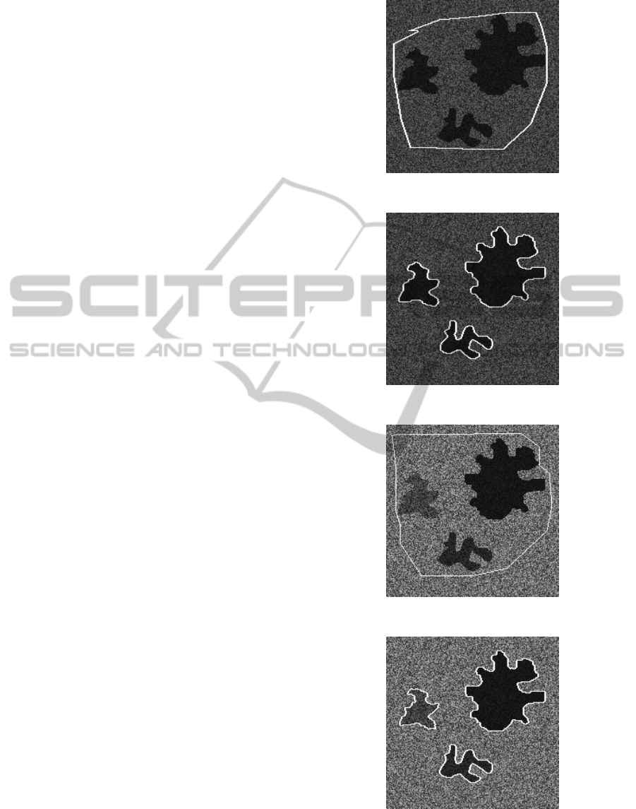
In Fig. 2 we can see the result obtained from

synthetic images constituted by background and three

objects to be extracted. This image is corrupted by

speckle noise of variance = 0.2. In Fig. 2, (a) and (b)

the objects have the same gray levels, whereas (c) and

(d) have three different gray levels. In Fig. 2, (b) and

(d) the results have been obtained by setting α = 0.5

and λ = 0.3.

In Fig. 3 we can see the overlapping of the results,

in particular in Fig. 3 (a) the contours have a distance

H = 4. and in Fig. 3 (b) H = 7.

4.2 Application to SAR Images

In this section we present some results performed by

applying the combined procedure on SAR images ac-

quired during ERS2 mission (2000).

ERS2 SAR system is capable of 25 m. resolution

from an altitude of 800 km, at radar wavelength of

5.7 cm.

In Fig. 4 the SAR images, representing part of the

coast of the Netherlands and a Baleari Island, are pre-

sented and the results obtained applying the level set

procedure, based on combined speed, are shown.

In Fig. 4 (a) we notice an image with inho-

mogeneities regarding the intensity within the fore-

ground. We used α = 0.6 and λ = 0.3. The ﬁnal re-

sult identiﬁes three islands and the coast. In this case

is important to underline that more objects are seg-

mented also in SAR images. In Fig. 4 (b) we note an

image with a granular aspect, small contrast between

foreground and background. We used α = 0.5 and

λ = 0.3.

In Fig. 5 the result, obtained on a SAR image of

750× 750 pixels, representing part of the coast of the

Tuscan coast, is shown. The result is characterized by

indented contour and by little islands and α = 0.5 and

λ = 0.3.

Fig. 6 shows the result obtained on a SAR image

of 500 × 700 pixels depicting the Capraia Island for

α = 0.3 and λ = 0.3.

An example of indented contour is in Fig. 7,

that shows the result obtained on a SAR image of

600×600 pixels representing part of the coast of Elba

Island, setting α = 0.5 and λ = 0.3

In the Fig. 8 (a) we present the image of size 200×

(a) Initial curve

(b) Final Contours

(d) Final contours

Figure 2: Speckled test images (200×200): (a) and(b)three

objects of the same gray level, (c)and (d) of different gray

levels

SpeckledImagesSegmentationandAlgorithmComparison

115

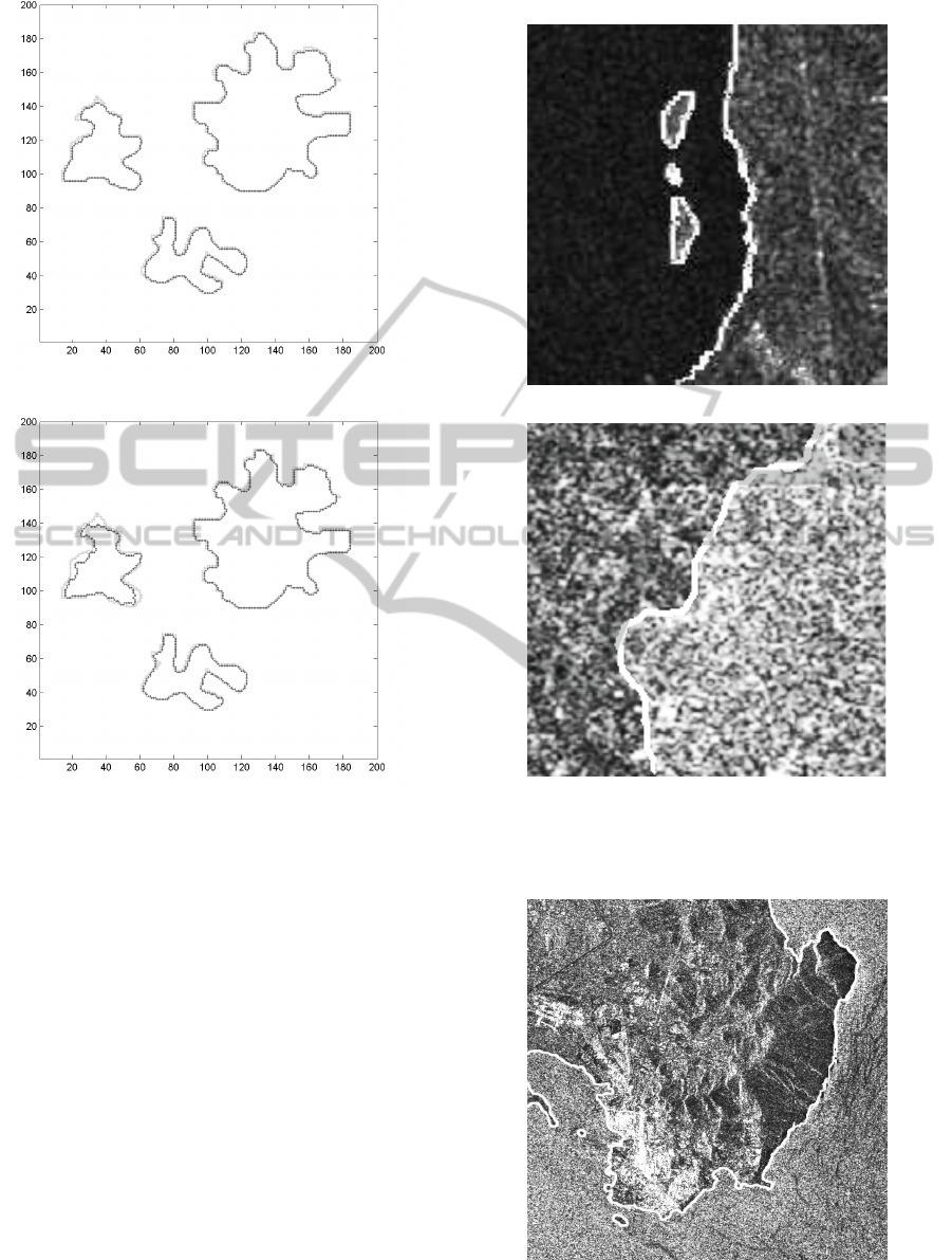
(a) H=4.

(b) H=7.

Figure 3: Hausdorff distance.

200 characterized by indented contour, representing

the Netherlands coast. The white line is portion of the

starting contour. The result of Fig. 8 (b) is obtained

for α = 0.4

The ﬁnal results is more than satisfactory.

5 CONCLUSIONS

In this paper, we presented a level set segmentation

algorithm applied to both synthetic and real SAR im-

ages and we discussed performance evaluation re-

sults.

The segmentation algorithm, based on a speed

balancing both the average and the gradient speeds,

works better than ones driven mainly by a single sep-

arated speed.

Combining two different speed functions for

(a) Regular contours

(b) Inhomogeneous background

Figure 4: Contours extraction of SAR images: (a) Nether-

lands coast and (b) Baleari coast.

Figure 5: Contour extraction from the Tuscan image, α =

0.5.

ICPRAM2015-InternationalConferenceonPatternRecognitionApplicationsandMethods

116

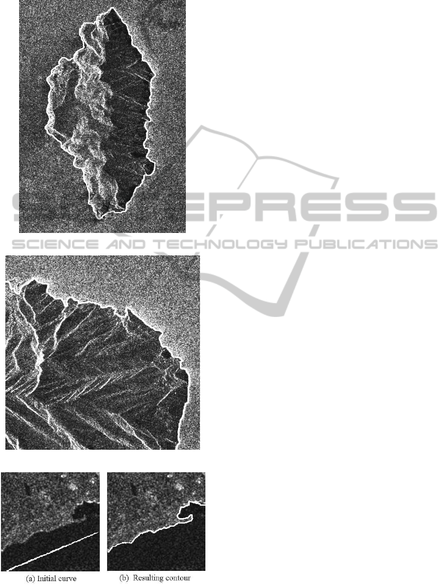
Figure 6: Contour extraction of the Capraia Island, α = 0.3.

Figure 7: Resulting contour of the Elba Island, α = 0.5.

Figure 8: Extraction contour: (a) original image and starting

contour, b) ﬁnal contour, α = 0.4.

curve evolution level set allows more accurate

achievements of regions contours. We compared the

results obtained applying the level set algorithm for

the speckled test and real images segmentation. Re-

sults appear to be very promising for future develop-

ments.

In the future we plan to apply the proposed method-

ology to full resolution images obtained from (CSK)

COSMO-SkyMed constellation. The constellation

consists of 4 satellites, each one equipped with a mi-

crowave high-resolution synthetic aperture radar. It

is the most important Italian event in the Space-Earth

Observation environment in international ﬁeld. We

are going to test and validate the proposed procedure

on images of the same regions acquired by different

SAR systems.

REFERENCES

Cinque, L. and Cossu, R. (2011). Region segmentation from

SAR images Lectures Notes Computer Science LNCS

6978 (ICIAP 2011), SPRINGER.

Sethian, J. A. (1999) Level set methods and fast marching

methods, Cambridge University Press, 1999.

Sethian, J. A. (2001) Evolution, implementation and ap-

plication of level set and fast marching methods for

advancing front, Journal of Computational Physics,

169 (2001).

Osher, S. and Fedkiw, R. (2002) Level set methods and

dynamic implicit surfaces, Springer-Verlag New York,

2002.

Ben Ayed, I. Mitiche, A. and Belhadj, Z. (2005), Multire-

gion level-set partitioning of synthetic aperture radar

images, IEEE Trans. Pattern Analysis and Machine

Intelligence, 27 (2005).

Mitiche, A. and Ben Ayed, I. (2011), Variational and

level set methods in image segmentation, (2011)

SPRINGER.

Ben Salah, M. Ben Ayed, I. and Mitiche, A. (2012), Ac-

tive curve recovery of region boundary patterns, IEEE

Trans. Pattern Analysis and Machine Intelligence, 34

(2012).

Yongjian, Yu and Acton Scott, T.(2002), Speckle reducing

anisotropic diffusion, IEEE Trans. on Image Process-

ing, 11 (2002).

Huttenlocher, D. Klanderman, G. and Rucklidge W. (1993)

Comparing Images Using the Hausdorff Distance,

IEEE Trans. Pattern Analysis Machine Intelligence,15

(1993).

Mumford, D. and Shah, J. (1989), Optimal approximations

by piecewise smooth functions and associated varia-

tional problems, Comm. Pure Appl.Math., 42 (1989).

Spitaleri, R. M. March, R. and Arena D. (1999), Finite

difference solution of Euler equation arising in varia-

tional image segmentation, Numerical Algorithms, 21

(1999).

SpeckledImagesSegmentationandAlgorithmComparison

117

Cinque, L. Cossu, R. and Spitaleri, R.M. (2014), Applied

variational SAR image segmentation, MASCOT12

& ISGG12 Proceedings, IMACS Series in Computa-

tional and Applied Mathematics,18 (2014).

Chan, T. F. and Vese, L. A. (2001), Active Contours without

edge, IEEE Trans. on Image Processing, 10 (2001).

Kass, M. Witkin, A. and Terzopoulos D. (2001), Snakes:

active contour models, Journal of Computational Vi-

sion, 1 (1988).

Cerimele, M.M. Cinque, L. and Cossu, R. (2009), Coast-

line detection from SAR images by level set model,

Lectures Notes Computer Science LNCS 5716 (ICIAP

2009), SPRINGER.

Perona, P. and Malik, J.,(1990) Scale space and edge detec-

tion using anisotropic diffusion, IEEE Trans. Pattern

Analysis and Machine Intelligence, 12 (1990).

Li, C. Xu, C. Gui and Fox, D. (2010), Distance regular-

ized level set evolution and its application to image

segmentation, IEEE Trans. on Image Processing, 11

(2010).

ICPRAM2015-InternationalConferenceonPatternRecognitionApplicationsandMethods

118