Relative Position Descriptors
A Review
M. Naeem and P. Matsakis
School of Computer Science, University of Guelph, Guelph, Canada
Keywords: Image Descriptors, Relative Position Descriptors, Spatial Relationships, Affine Invariance.
Abstract: A relative position descriptor is a quantitative representation of the relative position of two spatial objects. It
is a low-level image descriptor, like colour, texture, and shape descriptors. A good amount of work has been
carried out on relative position description. Application areas include content-based image retrieval, remote
sensing, medical imaging, robot navigation, and geographic information systems. This paper reviews the
existing work. It identifies the approaches that have been used as well as the properties that can be expected
from relative position descriptors. It compares and provides a brief overview of various descriptors,
including their main properties, strengths and limitations, and it suggests areas for future work.
1 INTRODUCTION
Relative position refers to the arrangement of objects
in space relative to each other. In daily life,
knowledge about relative positions is conveyed
through linguistic expressions like, “object A is
mostly above object B,” “object A is quite far from
object B,” or “object A almost touches object B.”
Such qualitative statements use terms that denote
spatial relationships, which are often categorized
into directional (e.g., above), distance (e.g., far) and
topological (e.g., touches) relationships. Relative
position information is important in various areas of
image processing and computer vision. However,
many practical image processing and computer
vision tasks call for quantitative measurements.
Quantitative models of relative position have
therefore been proposed. We call such models
relative position descriptors. They are visual
descriptors, like color, texture, and shape
descriptors, but they also intend to serve as
containers for spatial relationships. They therefore
provide a link between low-level spatial data
features and high-level concepts. The ideal relative
position descriptor gives a snapshot of the
arrangement of objects in space relative to each
other, it encapsulates rich information about all
kinds of spatial relationships between the objects,
and it allows this information to be easily extracted.
Relative position descriptors have received good
attention in image processing research in recent
years, as they have applications in object
recognition, image retrieval and indexing, map-to-
image conflation, linguistic scene description, etc.
Most of the attention has been focused on finding
effective approaches to the modeling of relative
positions and techniques for extracting spatial
relationship information from relative position
descriptors. Other topics that have received some
attention include the design of efficient algorithms;
the handling of fuzzy objects, objects in vector form,
and 3D objects; similarity and affine invariance.
There are several review papers on models of
spatial relationships (and these models may or may
not be based on relative position descriptors). See,
e.g., (Bloch, 2005) (Jaworski and Kucharski, 2010).
However, to our knowledge, this is the first review
paper on relative position descriptors. Section 2
identifies the approaches that have been used as well
as the properties that can be expected from these
descriptors. It also provides a summary of the
properties of various descriptors. Section 3 briefly
presents each descriptor mentioned in Section 2.
Conclusions are drawn in Section 4.
2 APPROACHES & PROPERTIES
2.1 Approaches
Table 1 indicates the approaches used to define the
286
Naeem M. and Matsakis P..
Relative Position Descriptors - A Review.
DOI: 10.5220/0005211002860295
In Proceedings of the International Conference on Pattern Recognition Applications and Methods (ICPRAM-2015), pages 286-295
ISBN: 978-989-758-076-5
Copyright
c
 2015 SCITEPRESS (Science and Technology Publications, Lda.)

relative position descriptors considered in this paper.
More on the definition of each descriptor can be
found in Section 3. The information necessary to fully
understand these table and section is presented below.
An object is a nonempty, regular closed subset of
the Cartesian plane. A pixel is a unit square whose
sides are parallel to the x- and y-axes and whose
center has integer coordinates. A raster object is the
union of a finite number of pixels. A vector object is
an object whose boundary is the union of a finite
number of line segments. Consider two objects A
and B. The position of A relative to B is usually
represented by a histogram H
AB
, or by a real
function improperly called a histogram, or by a tuple
of such functions. A working assumption is that the
objects may be too close to each other to be
approximated by their centroids or minimum
bounding boxes.
In the pixel-pair-based approach, the relative
position descriptor is designed with raster objects in
mind. A histogram value depends on pairs of pixels,
where each pair is composed of a pixel of A and a
pixel of B. In the point-pair-based approach, the
descriptor is designed with both raster and vector
objects in mind. A histogram value depends on pairs
of points, where each pair is composed of a point of
A and a point of B. In the segment-pair-based
approach, a histogram value depends on pairs of
aligned segments, where each pair is composed of a
segment of A and a segment of B. In the core-pair-
based approach, a histogram value depends on pairs
of aligned cores, where each pair is composed of a
core of A and a core of B. A core of an object is the
intersection of that object with a line.
The ϕ-histogram (Matsakis, Wendling and Ni,
2010) is a generic relative position descriptor
defined using the point-pair-based approach. The
symbol ϕ denotes a function that maps any triple
like (θ,p,q) to a real number, where p and q are
points and θ is a direction in the plane, i.e., θ is an
element of the interval (−π,π]. The histogram value
ϕ
AB
(θ) is the sum (integral) of all the ϕ(θ,p,q) values,
where p belongs to A and q to B. The F-histogram is
defined using the core-pair-based approach. F
denotes a function that maps any triple like (θ,I,J) to
a real number, where θ is a direction in the plane and
I and J are unions of aligned segments. The
histogram value F
AB
(θ) is the sum of all the F(θ,I,J)
values, where I is a core of A and J a core of B
aligned with I. Likewise, the f-histogram is defined
using the segment-pair-based approach. f denotes a
function that maps any triple like (θ,I,J) to a real
number, where I and J are aligned segments.
Table 1: Approaches.
DESCRIPTOR
APPROACH
pixel/point/segment/core-pair-based
APPROACH
boundary/region-based
generic
ϕ-histogram
point-pair-based region-based
f-histogram
segment-pair-based region-based
F-histogram
core-pair-based region-based
specific
angle histogram
pixel-pair-based region-based
force histogram
point-pair-based
(ϕ-histogram)
region-based
Allen histograms
core-pair-based
(F-histogram)
region-based
R-histogram
pixel-pair-based boundary-based
R*-histogram
pixel-pair-based region-based
spread histogram
pixel-pair-based region-based
visual area histogram
pixel-pair-based boundary-based
radial line model
core-based
region-based
ratio histogram
core-
p
ai
r
-
b
ase
d
(F-function-based)
region-based
RelativePositionDescriptors-AReview
287

Moreover, a relative position descriptor may be
defined using a region-based approach (all the
pixels, or all the points of the objects are considered)
or a boundary-based approach (only the boundary
pixels, or the boundary points, are considered).
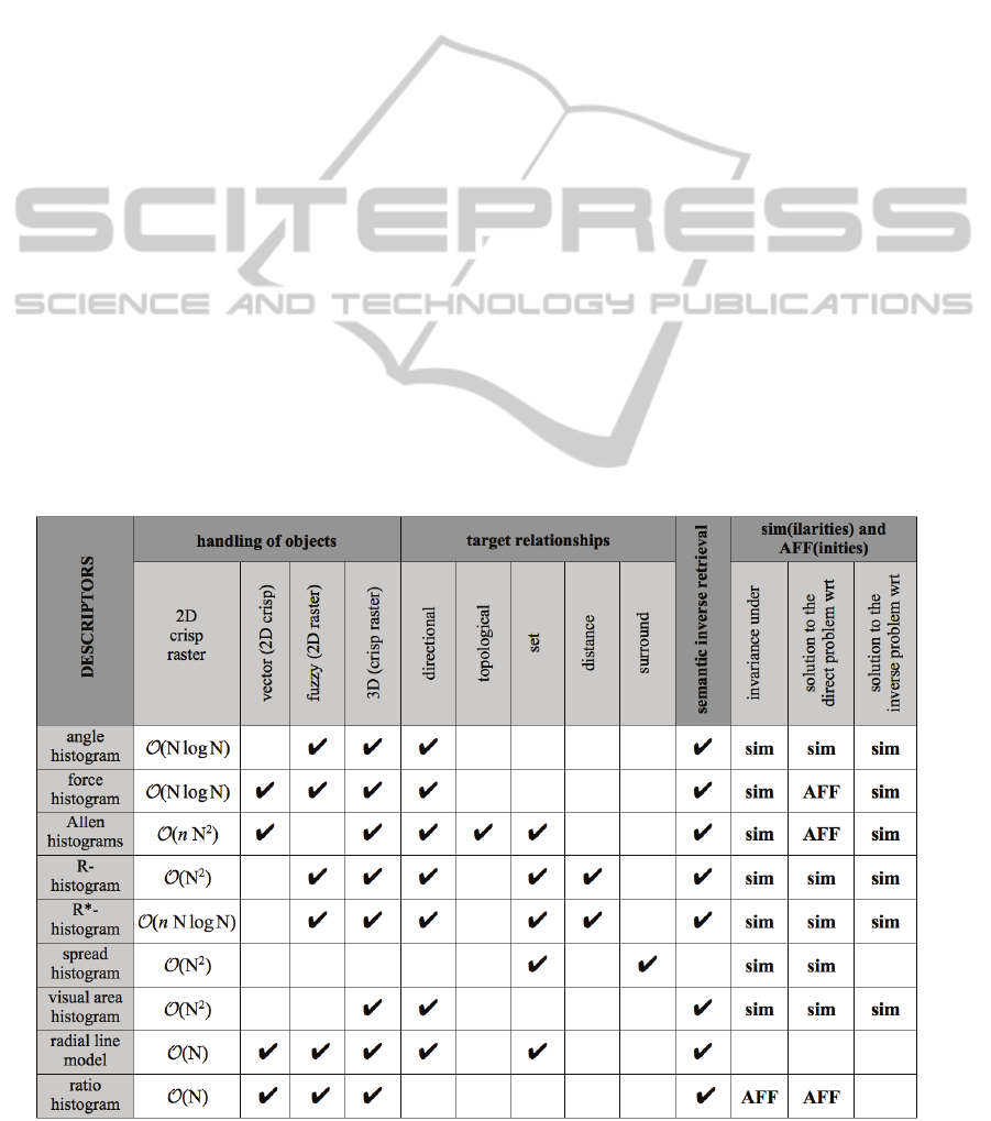
2.2 Properties
Table 2 summarizes the properties and
characteristics of the relative position descriptors
considered in this paper. More about the properties
and characteristics of each descriptor can be found
in Section 3. The information necessary to fully
understand these table and section is presented
below.
An object as defined in Section 2.1 is a 2D crisp
object. From now on, unless otherwise specified,
objects will be assumed to be raster objects. All
relative position descriptors can handle (2D crisp
raster) objects without having to vectorize them.
Likewise, we say that a descriptor can handle (2D
crisp) vector objects if there is no need to rasterize
them. We say that a descriptor can handle (2D)
fuzzy (raster) objects if there is no need for a general
and computationally expensive approach like the
double sum or simple sum scheme (Dubois and
Jaulent, 1987) (Krishnapuram et al., 1993).
The symbol N refers to the number of pixels in
the image (case of raster objects), and n is the
number of directions θ considered (case of
histograms defined on the set (−π,π] of directions in
the plane). When dealing with raster objects, n is
Ο(√N) at worst and Ο(1) at best. Practically, there
does not seem to be any interest in considering more
than a few hundred directions, whatever N.
A relative position descriptor is usually designed so
that specific spatial relationship information can be
extracted. The target relationships can be directional,
topological, or distance relationships. Note that
topological relationships include set relationships.
For example, the condition A∩B≠∅ defines the set
(and hence topological) relationship intersects,
while A∩B≠∅ and int(A)∩int(B)=∅ define the
topological (but non-set) relationship touches.
Surroundedness is treated independently. The fact
that the target relationships are, say, topological,
does not mean of course that information about every
possible topological relationship can be extracted, and
there is no implication about the quality (e.g.,
completeness, meaningfulness) of the extracted
information. Moreover, a descriptor may allow some
information about non-target relationships to be
extracted.
Table 2: Properties. An empty cell means that, to our knowledge, the property has not been investigated, and that, as far as
we can tell, there is no straightforward evidence towards the property.
ICPRAM2015-InternationalConferenceonPatternRecognitionApplicationsandMethods
288

Affine or similarity invariant descriptors play an
important role in image processing and computer
vision. Examples of similarity invariant colour,
texture, and shape descriptors abound in the
literature. Consider a geometric transformation t.
We say that the relative position descriptor H is
invariant under t if for any objects A and B we have
H
t(A)t(B)
= H
AB
. If H is not invariant under t, there may
be a normalization procedure H
AB
a
H
AB
such
that
H
t (A)t (B)
=
H
AB
=
H
A' B'
, where the objects A'
and B' can be derived from A and B using some
invertible transformation. The normalized descriptor
is then invariant under t. Note that all the descriptors
considered in this paper are invariant under
translations.
It may be possible to find H
t(A)t(B)
knowing t and
H
AB
, without having to rely on any computational
optimization technique. We then say that the
descriptor offers a solution to the direct problem
with respect to t, or that the behaviour of the
descriptor under t is known. It may also be possible
to find t (up to a translation) knowing H
AB
and
H
t(A)t(B)
. We then say that the descriptor offers a
solution to the inverse problem with respect to t.
Finally, it may be possible to find H
BA
knowing H
AB
.
We then say that the descriptor allows semantic
inverse retrieval.
3 DESCRIPTORS
Here, we briefly present the descriptors mentioned
in Section 2. We also comment on some of their
properties (which are listed in Table 2).
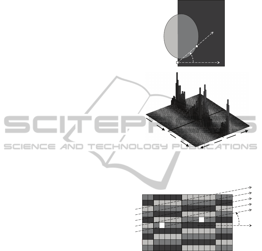
3.1 Angle Histogram
Consider two raster objects A and B (Fig. 1a). For
any pixels p of A and q of B, with p≠q, let ∠(p,q) be
the angle between the x-axis and the directed line
that passes through the center of q and then of p.
This angle belongs to (−π,π]. Partition (−π,π] into n
intervals Θ
1
, Θ
2
, etc. (the direction bins). The
histogram value H
AB
(i) is the number of pixel pairs
(p,q)∈A×B such that ∠(p,q)∈Θ
i
. See (Krishnapuram
et al., 1993) (Miyajima and Ralescu, 1994).
Note
The histogram of angles may be the first true relative
position descriptor. The original algorithm runs in
Ο(N
2
) time. To shorten processing times, it is of
course possible to downsize the image before
computing the histogram. A similar approach is to
partition each object into rectangular blocks of
pixels and to consider that the center of any pixel in
a given block is the center of the block. This is the
principle of a variant of the histogram of angles
called the quadtree histogram (Wang, 2013) (Zhang
et al., 2014). Also note that the histogram of angles
can be computed in Ο(N
log N) time using the same
Ο(N
log N) approach as for force histograms
(Matsakis, Wendling and Ni, 2010). Nonetheless,
processing times are usually much longer than for
other relative position descriptors.
Directional relationship information can be
extracted using, e.g., the aggregation (Krishnapuram
et al., 1993) or the compatibility method (Miyajima
and Ralescu, 1994).
At first glance, the behaviour of the histogram
under similarity transformations seems easy to
determine and similarity invariance seems easy to
obtain. This, however, may not be the case. One issue
is how to choose the number of bins, n. For example,
if the bins are too narrow then the histogram of
angles inherits the anisotropy of the grid of pixels.
Let rot be a π/4-angle rotation. Assume 0∈Θ
i
and
π/4∈Θ
j
. We should have H
rot(A)rot(B)
(j) ≈ H
AB
(i).
Instead, we get H
rot(A)rot(B)
(j) ≈ H
AB
(i)/√2.
(a)
(b)
Figure 1: Histogram of angles. (a) H
AB
(i) is the number
of pixel pairs (p,q) such that θ falls into Θ
i
. (b) Example.
i
H
AB
(i)
RelativePositionDescriptors-AReview
289

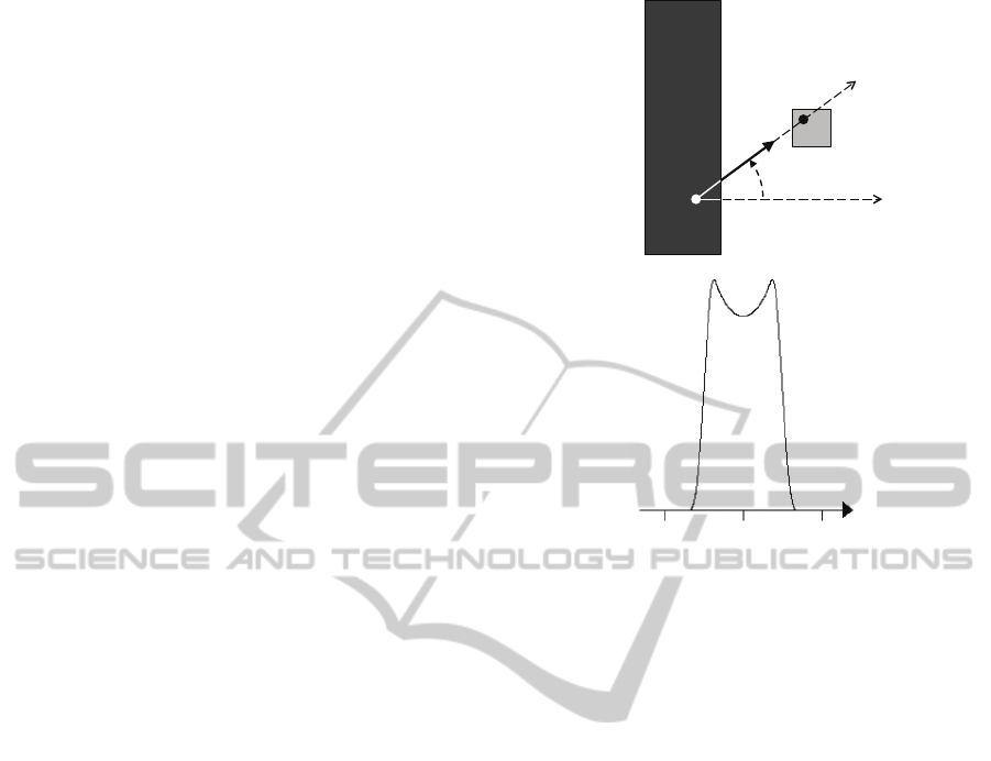
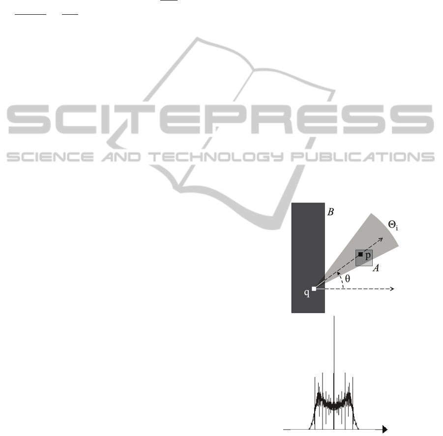
3.2 Force Histogram
The histogram of forces (Matsakis and Wendling,
1999) is a ϕ-histogram. Consider two objects A and
B and two points p∈A and q∈B, as in Fig. 2a. Let qp
be the vector from q to p and let |qp| be its length. A
function ϕ, denoted by ϕ
r
, is attached to the real
number r. It maps (θ,p,q) to 1/|qp|
r
if θ is the
direction of qp and to 0 otherwise. p and q are seen
as particles and the vector qp/|qp|
r+1
as an
elementary force exerted by p on q. The histogram
value
ϕ
r
AB
(θ)
is then the scalar resultant of all the
elementary forces in direction θ.
Note
When r=2, the forces are gravitational-like. When
r=0, the forces are distance-independent, and the
histogram of forces coincides with (but does not
have the weaknesses of) the histogram of angles.
The original algorithm runs in Ο(nN√N) time,
where n is the number of directions θ considered.
The best case performance (convex objects) is Ο(nN).
A more recent algorithm (Matsakis, Wendling and
Ni, 2010) runs in Ο(N
log N), but the processing
times are usually much longer, unless n is very large
or the objects are fractal-like.
Directional relationship information can be
extracted using the same methods as for the
histogram of angles, or using a method based on
force categorization (Matsakis, Wendling and Ni,
2010).
Fuzzy objects and 3D objects are best handled by
the Ο(N
log N) algorithm. Vector objects can be
handled as well (Recoskie et al., 2012). However,
the time complexity of the algorithm has been
severely underestimated and is Ο(n
η
3
) instead of
Ο(n
η log η), where η is the total number of object
vertices. The best case performance (convex objects)
is Ο(n
η
2
).
The histogram of forces has found many
applications, including human-robot interaction
(Skubic et al., 2004), geospatial information retrieval
and indexing (Shyu et al., 2007), and map-to-image
conflation (Buck et al., 2013).
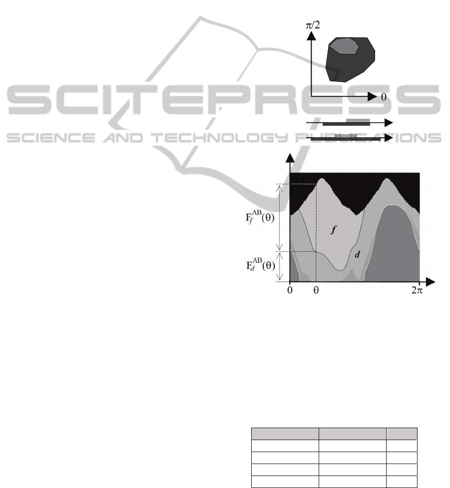
3.3 Allen Histograms
The Allen histograms are a tuple of 13 F-histograms
(Malki et al., 2002) (Matsakis and Nikitenko, 2005).
Allen’s logic considers 13 jointly exhaustive and
pairwise disjoint relations for convex temporal in-
(a)
(b)
Figure 2: Histogram of forces. (a)
ϕ
r
AB
(
θ
)
is the sum
(integral) of all the elementary forces in direction θ. (b)
Example.
tervals (Allen, 1983). Each relation r corresponds to
a topological relationship between two segments on
a directed line. A function F, denoted by
F
r
, is
attached to r. It extends r from pairs of segments to
pairs of cores, while the Allen histogram
F
r
AB
extends r from pairs of segments to the pair (A,B) of
objects.
F
r
AB
(
θ
)
measures the extent to which r
holds, in direction θ, between A and B. See Fig. 3.
First, r is fuzzified. r(I,J), where I and J are two
segments on a directed line, denotes a real number
between 0 (it is totally false that r holds between I
and J) and 1 (it is totally true). For example, if two
segments are disjoint but very close to each other,
then we want to be able to say that they almost
touch. Next, the cores of the objects are fuzzified as
well. The idea is to consider that if two segments in
a core are very close, then they should be seen, to a
certain extent, as a single segment. Now, consider a
line L in direction θ. Any α-cut of the fuzzy core
A∩L is the union of pairwise disjoint segments
I
i
α
.
Likewise, any α-cut of B∩L is the union of
segments
J
j
α
. The function
F
r
maps (θ, A∩L, B∩L)
to a weighted average of all the r(
I
i
α
,
J
j
α
).
Note
The idea of using 13 histograms, 1 per Allen
p
q
θ
A
B
-π/2 0 π/2
θ
φ
AB
(θ)
0
ICPRAM2015-InternationalConferenceonPatternRecognitionApplicationsandMethods
290

relation, to describe the relative position of objects
was first proposed by Malki et al. (2002). Only
convex objects can be handled, and there is no
consistency between the histograms⎯which are f-
histograms. The idea was revisited by Matsakis and
Nikitenko (2005) to address these flaws. The f-
histograms are replaced with F-histograms. The
worst case performance is Ο(nN
2
). The best case
performance (convex objects) is Ο(nN).
The definition of the Allen F-histograms was
simplified and adapted to the handling of vector
objects by Salamat and Zahzah (2012a). However,
the time complexity of the algorithm was severely
underestimated. It is Ο(n
η
3
) instead of Ο(n η log η),
where η is the total number of object vertices. The
best case performance (convex objects) is Ο(n
η
2
).
There is a straightforward extension to 3D objects,
but processing times are prohibitive.
Meaningful directional and topological
relationship information can be extracted when the
objects are convex (Salamat and Zahzah, 2012b),
but is much harder to extract when the objects are
concave (Matsakis, Wawrzyniak and Ni, 2010)
because of the inadequacy of describing 2D spatial
relationships in terms of Allen’s 1D temporal
relationships (Cohn et al., 1997).
The Allen histograms have been used for
linguistic scene description (Matsakis, Wawrzyniak
and Ni, 2010), spatio-temporal reasoning (Salamat
and Zahzah, 2012c) and the modeling of motion
classes (Salamat and Zahzah, 2012d).
3.4 R-Histogram
Consider two raster objects A and B. For any pixels
p of A and q of B, let ∠(p,q) be the angle between
the x-axis and the directed line that passes through
the center of q and then of p, let d(p,q) be the
distance from p to q, and let l(p,q) be the integer as
defined in Table 3. See Fig. 4. The angle ∠(p,q) is an
element of (−π,π] while d(p,q) belongs to some
interval [0, d
max
]. Partition (−π,π] into n intervals Θ
1
,
Θ
2
, etc. (the direction bins), and partition [0, d
max
]
into m intervals D
1
, D
2
, etc. (the distance bins). The
histogram value R
AB
(i,j,k) is the number of pixel
pairs (p,q) such that:
p is a boundary pixel of A,
q is a boundary pixel of B,
∠(p,q)∈Θ
i
and d(p,q)∈D
j
and l(p,q)=k.
See (Wang and Makedon, 2003).
Note
While the worst case performance is Ο(N
2
), the best
case performance (convex objects) is Ο(N).
The R-histogram obviously supports extraction
of some directional, set and distance relationship
information, but extraction methods and models of
spatial relationships based on the R-histogram have
not been investigated.
The R-histogram can only handle objects that are
homeomorphic to a 2-ball. There are straightforward
extensions to fuzzy objects and 3D objects, but
processing times may be prohibitive.
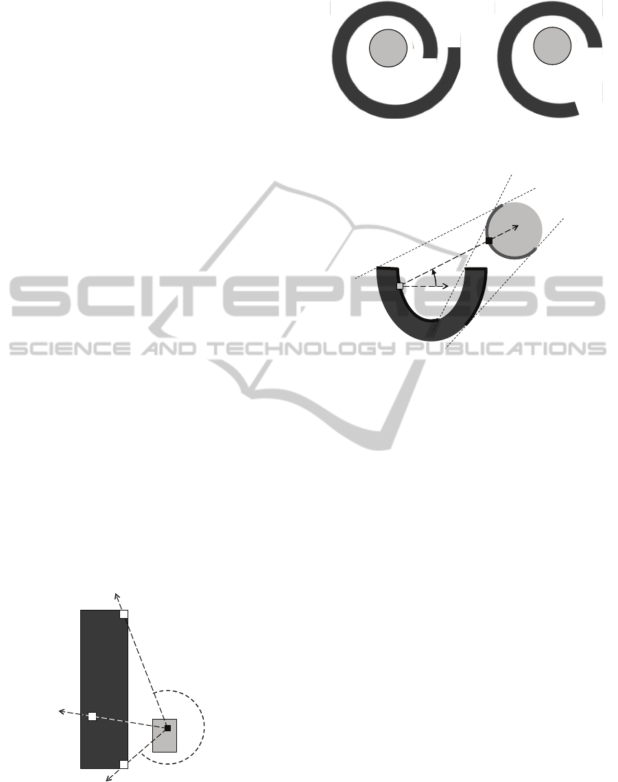
(a)
(b)
(c)
Figure 3: Allen histograms. (a) A pair of objects. (b) The
Allen relations f (finishes) and d (during). (c) The 13 Allen
histograms associated with (A,B) and stacked on top of
each other.
The behaviour of the R-histogram under similarity
transformations seems easy to determine and
similarity invariance seems easy to obtain. However,
see last paragraph of Section 3.1.
Table 3: The label l(p,q).
p is a pixel of B q is a pixel of A l(p,q)
false false 0
true false 1
false true 2
true true 3
The R-Histogram has been applied to similarity-
based image retrieval.
B
A
d
f
RelativePositionDescriptors-AReview
291

3.5 R*-Histograms
Consider two raster objects A and B and an element
θ of the interval (−π,π]. The image is partitioned into
raster lines running in direction θ, as shown in Fig.
5. For any pixels p of A and q of B, let d(p,q) be the
distance from p to q, and let l(p,q) be the integer as
in Table 3. The distance d(p,q) belongs to some
interval [0,d
max
]. Partition [0,d
max
] into m intervals
D
1
, D
2
, etc. (the distance bins). The histogram value
R*
AB
(θ,j,k) is the number of pixel pairs (p,q)∈A×B
such that:
q is before p on the same raster line,
d(p,q)∈D
j
and l(p,q)=k.
See (Wang et al., 2004).
Note
A first algorithm runs in Ο(n N √N) time, where n is
the number of directions θ considered. A second
algorithm runs in Ο(n
N log N). No comparative
study of the two algorithms is available.
Extension to vector objects may be possible.
There are straightforward extensions to fuzzy
objects and 3D objects, but processing times may be
prohibitive.
The R*-histogram obviously supports extraction
of some directional, set and distance relationship
information, but extraction methods and models of
spatial relationships based on the R*-histogram have
not been investigated.
The R*-histogram probably offers a solution to
the direct and inverse problems with respect to affine
transformations (as long as the distance d
max
is
determined independently for each direction θ and
recorded). A normalization procedure should then
allow affinity invariance. These issues deserve further
investigation.
3.6 Spread Histogram
Consider two raster objects A and B, as in Fig. 6. For
any pixel p of A, the half-lines originating from the
centre of p and passing through the centres of the
pixels of B divide the plane into sectors. Let ∠(p,B)
be the central angle of the largest sector. This angle
belongs to [0,2π]. Now, partition [0,2π] into n
intervals Θ
1
, Θ
2
, etc. The value H
AB
(i) is the number
of pixels p∈A such that ∠(p,B)∈Θ
i
. See (Kwasnicka
and Paradowski, 2005).
(a)
(b)
Figure 4: R-histogram. (a) R
AB
(i,j,k) is the number of
boundary pixel pairs (p,q) such that the angle θ falls into
the bin Θ
i
, the distance d(p,q) falls into the bin D
j
and
l(p,q)=k. (b) Representation.
Figure 5: R*-histogram. The image is partitioned into
raster lines running in direction θ. Here, the pixels p and q
are on the same raster line, and q is before p.
Note
The spread histogram is meant to be used along with
the histogram of angles. The two can be computed
simultaneously in Ο(N
2
) time and allow extraction
of directional relationship information as well as
information on the relationships inside (A⊆B),
outside (A∩B=∅) and surround. Note that, here,
surroundedness should be understood as visual
surroundedness (Rosenfeld and Klette, 1984), not as
topological surroundedness. See Fig. 7.
The behaviour of the spread histogram under
similarity transformations seems easy to determine
q
p
B
A
θ
k=2
k=3
k=0
k=1
i
i
j
j
θ
p
q
ICPRAM2015-InternationalConferenceonPatternRecognitionApplicationsandMethods
292

and similarity invariance seems easy to obtain.
However, see last paragraph of Section 3.1.
3.7 Visual Area Histogram
Consider two disjoint raster objects A and B, as in
Fig. 8. For any pixels p of A and q of B, if a raster
segment whose endpoints are p and q does not
contain any other pixel of A or B then p is a
boundary pixel of A visible from B and q is a
boundary pixel of B visible from A. Let ∠(p,q) be
the angle between the x-axis and the directed line
that passes through the center of q and then of p.
This angle belongs to (−π,π]. Partition (−π,π] into n
intervals Θ
1
, Θ
2
, etc. The histogram value H
AB
(i) is
the number of pixel pairs (p,q) such that
p is a boundary pixel of A visible from B,
q is a boundary pixel of B visible from A,
and ∠(p,q)∈Θ
i
.
There is, however, a more general definition. Instead
of contributing 1 unit to H
AB
(i), a pair (p,q) as above
may contribute [d
min
/ d(p,q)]
r
, where r is a real
number, d(p,q) is the distance from p to q, and d
min
is
the minimum distance over all pairs. See (Zhang et
al., 2010).
Note
The visual area histogram can only handle disjoint
objects. The algorithm runs in Ο(N
2
) time. In most
cases, however, computing a visual area histogram is
expected to be much faster than computing a
histogram of angles, since many fewer pixel pairs
are considered.
There is a straightforward extension to 3D objects,
but processing times may be prohibitive.
The behaviour of the visual area histogram under
Figure 6: Spread histogram. The half-lines originating from
the centre of p and passing through the centres of the pixels
of B divide the plane into sectors. Here, the central angle
∠(p,B) of the largest sector is θ.
(a) (b)
Figure 7: Visual surroundedness. (a) A is completely
surrounded by B. (b) A is partially surrounded by B.
Figure 8: Visual area histogram. p is a boundary pixel of A
visible from B and q is a boundary pixel of B visible from A.
Here, ∠(p,q)=θ.
similarity transformations seems easy to determine
and similarity invariance seems easy to obtain.
However, see last paragraph of Section 3.1.
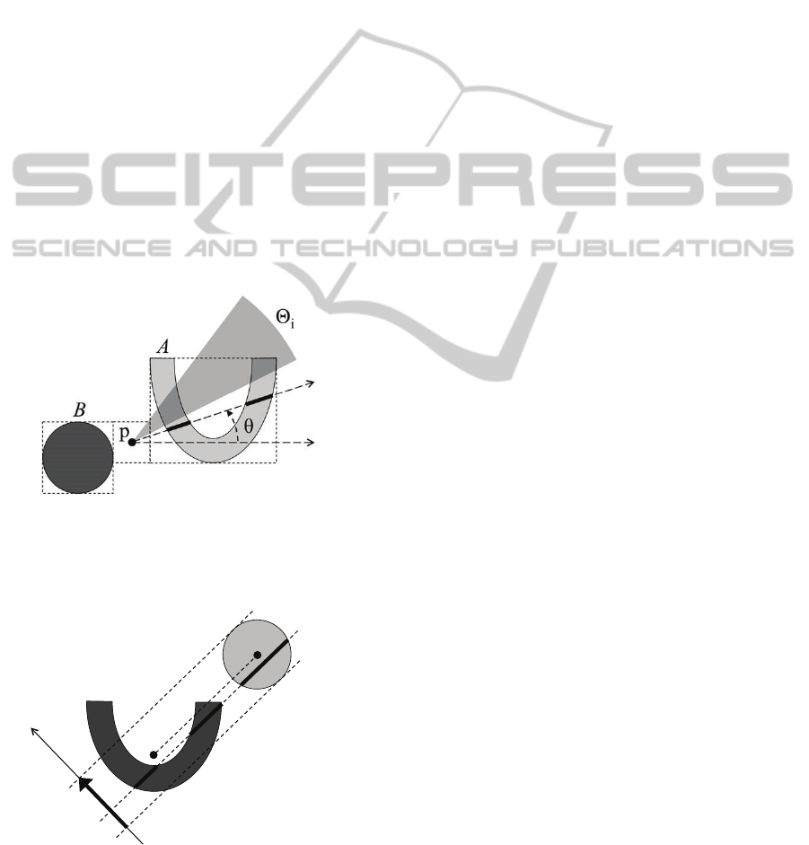
3.8 Radial Line Model
Consider two objects A and B, and a reference point
p determined by the minimum bounding rectangles
of the objects, as suggested in Fig. 9. Partition
(−π,π] into n intervals Θ
1
, Θ
2
, etc. (the direction
bins). The unbounded sector extending from p and
defined by Θ
i
intersects A (resp. B) in some region A
i
(resp. B
i
). The histogram value H
A
(i) (resp. H
B
(i)) is
the area of A
i
(resp. B
i
) over the area of A (resp. B).
The position of A relative to B is represented by the
pair (H
A
, H
B
). See (Santosh et al., 2010).
Note
The Radial Line Model (RLM) targets directional
and set relationships. However, extraction methods
and models of such relationships based on the RLM
have not been investigated. Besides, the RLM does
not always allow us to determine whether two
objects overlap, or whether one includes the other.
The behaviour of the RLM under similarity
transformations is unknown, and similarity
invariance cannot be obtained. These two properties
would hold, however, if the model was defined as
A
B
p
θ
A
B
A
B
A
B
p
q
θ
RelativePositionDescriptors-AReview
293

follows: choose p as the centroid of A∪B; the half-
line that extends from p in direction θ intersects A
(resp. B) in a union (possibly empty) of pairwise
disjoint segments (Fig. 9); set the histogram value
H
A
(θ) (resp. H
B
(θ)) to the total length of these
segments, and represent the position of A relative to
B by the pair (H
A
, H
B
).
The RLM has been used for graphical symbol
retrieval.
3.9 Ratio Histogram
Consider two objects A and B with distinct centroids
a and b. Any real number x can be mapped to a line
L(x) as shown in Fig. 10. This line L(x) is parallel to
the line that passes though a and b, it does not
intersect both objects if x is less than 0 or greater
than 1, and it does intersect both objects if x is 0 or
1. The core A∩L(x) is the union of a finite number of
pairwise disjoint segments. Let |A∩L(x)| be the total
length of these segments. The ratio histogram H
AB
is
the function x
a
|A∩L(x)| / |B∩L(x)|. See (Wang et
al., 2012).
Figure 9: Radial Line Model. H
A
(i) is the total area of the
two darker regions in A, divided by the area of A. Another
option is to define H
A
(θ) as the total length of the two black
segments.
Figure 10: Ratio histogram. The line L(x).
Note
The centroids of the two objects must be distinct.
The ratio histogram is designed to be invariant
to affine transformations. As a result, it offers a
trivial solution to the direct problem with respect to
affinities, and there is no solution to the inverse
problem with respect to similarities.
The ratio histogram has been used for shape
matching and object recognition.
4 CONCLUSIONS
Various relative position descriptors have been
considered in this review. They illustrate various
approaches to relative position description, and are
of interest for various reasons. For example, the
Allen histograms are the only ones that really target
topological relationships; the spread histogram is the
only one that targets surrounds; the ratio histogram
is the only one that is affine invariant. Every
descriptor has its strengths, and its limitations:
meaningful topological relationship information
cannot be easily extracted from Allen histograms
when the objects are concave; the spread histogram
is computationally expensive; the discriminating
power of the ratio histogram is low. There is a need
for a more versatile descriptor, that targets all types
of spatial relationships. Moreover, there is no
descriptor that offers a solution to the inverse
problem with respect to affine transformations, and
there is no descriptor that offers a solution to the
recovery problem (i.e., given a relative position
descriptor, find all the pairs of objects that receive
the same description). All these are potential areas
for future work.
REFERENCES
J. F. Allen, 1983. “Maintaining Knowledge About
Temporal Intervals,” Communications of the ACM,
26(11): 832-43.
I. Bloch, 2005. “Fuzzy Spatial Relationships for Image
Processing and Interpretation: A Review,” Image and
Vision Computing, 23(2):89-110.
A. Buck, J. Keller, M. Skubic, 2013. “A Memetic
Algorithm for Matching Spatial Configurations with
the Histograms of Forces,” IEEE Trans. on
Evolutionary Computation, 17(4):588-604.
A. G. Cohn, B. Bennett, J. Gooday, N. M. Gotts, 1997.
“Qualitative Spatial Representation and Reasoning
with the Region Connection Calculus,”
GeoInformatica, 1(3):275-316.
D. Dubois, M.-C. Jaulent, 1987. “A General Approach to
A
B
a
0
b
1
x
L(x)
ICPRAM2015-InternationalConferenceonPatternRecognitionApplicationsandMethods
294

Parameter Evaluation in Fuzzy Digital Pictures,”
Pattern Recognition Letters, 6:251-59.
T. Jaworski, J. Kucharski, 2010. “The Use of Fuzzy Logic
for Description of Spatial Relations between Objects,”
Automatyka, 14:563-80.
R. Krishnapuram, J. M. Keller, Y. Ma, 1993. “Quantitative
Analysis of Properties and Spatial Relations of Fuzzy
Image Regions,” IEEE Trans. on Fuzzy Systems, 1(3):
222-33.
H. Kwasnicka, M. Paradowski, 2005. “Spread Histogram
⎯ A Method for Calculating Spatial Relations
Between Objects,” 4th Int. Conf. on Computer
Recognition Systems (CORES), Proceedings, 30:249-
56.
J. Malki, E.-H. Zahzah, L. Mascarilla, 2002. “Indexation
et recherche d'image fondées sur les relations spatiales
entre objets,” Traitement du Signal, 18(4):235-51.
P. Matsakis, D. Nikitenko, 2005. “Combined Extraction of
Directional and Topological Relationship Information
from 2D Concave Objects,” in M. Cobb, F. Petry, V.
Robinson (Eds.), Fuzzy Modeling with Spatial
Information for Geographic Problems, Springer-
Verlag, 15-40.
P. Matsakis, L. Wawrzyniak, J. Ni, 2010. “Relative
Positions in Words: A System that Builds Descriptions
Around Allen Relations,” Int. J. of Geographical
Information Science, 24(1):1-23.
P. Matsakis, L. Wendling, 1999. “A New Way to
Represent the Relative Position of Areal Objects,”
IEEE Trans. on Pattern Analysis and Machine
Intelligence, 21(7):634-43.
P. Matsakis, L. Wendling, J. Ni, 2010. “A General
Approach to the Fuzzy Modeling of Spatial
Relationships,” in R. Jeansoulin, O. Papini, H. Prade,
S. Schockaert (Eds.), Methods for Handling Imperfect
Spatial Information, Springer-Verlag, 49-74.
K. Miyajima, A. Ralescu, 1994. “Spatial Organization in
2D Segmented Images: Representation and
Recognition of Primitive Spatial Relations,” Fuzzy
Sets and Systems, 65(2-3):225-36.
D. Recoskie, T. Xu, P. Matsakis, 2012. “A General
Algorithm for Calculating Force Histograms using
Vector.
Data,” 1st Int. Conf. on Pattern Recognition Applications
and Methods (ICPRAM), Proceedings, 86-92.
A. Rosenfeld, R. Klette, 1984. Degree of Adjacency or
Surroundedness, University of Maryland, 30 pages.
N. Salamat, E.-H. Zahzah, 2012a. “On the Improvement
of Combined Fuzzy Topological and Directional
Relations Information,” Pattern Recognition,
45(4):1559-68.
N. Salamat, E.-H. Zahzah, 2012b. “Two-Dimensional
Fuzzy Spatial Relations: A New Way of Computing
and Representation,” Advances in Fuzzy Systems,
2012:1-15.
N. Salamat, E.-H. Zahzah, 2012c. “Spatio-Temporal
Reasoning by Combined Topological and Directional
Relations Information,” Int. J. of Artificial Intelligence
and Soft Computing, 3(2):185-201.
N. Salamat, E.-H. Zahzah, 2012d. “Spatiotemporal
Relations and Modeling Motion Classes by Combined
Topological and Directional Relations Method,” ISRN
Machine Vision, 12 pages.
K.C. Santosh, L. Wendling, B. Lamiroy, 2010. “Unified
Pairwise Spatial Relations: An Application to
Graphical Symbol Retrieval”, in J.-M. Ogier, W. Liu,
J. Llados (Eds.), Graphics Recognition.
Achievements, Challenges, and Evolution, Springer-
Verlag, 163-74.
C.-R. Shyu, M. Klaric, G. J. Scott, A. S. Barb, C. H. Davis,
K. Palaniappan, 2007. “GeoIRIS: Geospatial
Information Retrieval and Indexing System ⎯ Content
Mining, Semantics Modeling, and Complex Queries,”
IEEE Trans. on Geoscience and Remote Sensing,
45(4):839-52.
M. Skubic, D. Perzanowski, S. Blisard, A. Schultz, W.
Adams, M. Bugajska, D. Brock, 2004. “Spatial
Language for Human-Robot Dialogs,” IEEE Trans. on
Systems, Man, and Cybernetics (Part C), 34(2):154-67.
Z. Wang, 2013. “A New Quadtree Histogram-Based Spatial.
Modeling Based on Cloud Model,” Int. J. of Hybrid
Information Technology, 6(6):31-40.
Y. Wang, F. Makedon, 2003. “R-Histogram: Quantitative
Representation of Spatial Relations for Similarity-
Based Image Retrieval,” ACM Int. Multimedia Conf.
and Exhibition (MM), Proceedings, 323-6.
Y. Wang, F. Makedon, A. Chakrabarti, 2004. “R*-
Histograms: Efficient Representation of Spatial
Relations between Objects of Arbitrary Topology,”
12th Annual Int. Conf. on Multimedia (MM),
Proceedings, 356-9.
W. Wang, B. Xiong, H. Sun, H. Cai, Y. Jiang, G. Kuang,
2012. “An Affine Invariant Relative Attitude
Relationship Descriptor for Shape Matching Based on
Ratio Histograms,” EURASIP J. on Advances in
Signal Processing, 2012(1):1-10.
K. Zhang, T. Liu, Z. Li, W. Zhao, 2014. “A New
Directional Relation Model,” Int. J. of Signal
Processing, Image Processing & Pattern Recognition,
7(2):237-48.
K. Zhang, K. Wang, X. Wang, Y. Zhong, 2010. “Spatial
Relations Modeling Based on Visual Area Histo-
gram,” 11th ACIS Int. Conf. on Software Engineering
Artificial Intelligence Networking and Parallel/Dis-
tributed Computing (SNPD), Proceedings, 97-101.
RelativePositionDescriptors-AReview
295