Analyzing the Effect of Lossy Compression on Particle Traces in

Turbulent Vector Fields

Marc Treib, Kai B

urger, Jun Wu and R

udiger Westermann

Technische Universit

at M

unchen, Munich, Germany

Keywords:

Vector Fields, Turbulence, Particle Tracing, Data Compression, Data Streaming.

Abstract:

We shed light on the accuracy of particle trajectories in turbulent vector ﬁelds when lossy data compression is

used. So far, data compression has been considered rather hesitantly due to supposed accuracy issues. Moti-

vated by the observation that particle traces are always afﬂicted with inaccuracy, we quantitatively analyze the

additional inaccuracies caused by lossy compression. In some experiments we conﬁrm that the compression

has only minor impact on the accuracy of the trajectories. Even though our experiments are not generally valid,

they indicate that a more thorough analysis of the error in particle integration due to compression is necessary,

and that in some cases lossy compression is valid and can signiﬁcantly reduce performance limitations due to

memory and communication bandwidth.

1 INTRODUCTION

One of the most intriguing and yet to be fully under-

stood aspects in turbulence research is the statistics of

Lagrangian ﬂuid particles transported by a fully de-

veloped turbulent ﬂow. Here, a ﬂuid particle is con-

sidered a point moving with the local velocity of the

ﬂuid continuum. The analysis of Lagrangian statis-

tics is usually performed numerically by following the

time trajectories of ﬂuid particles in numerically sim-

ulated turbulent ﬁelds. Let x(y, t) and u(y, t) denote

the position and velocity at time t of a ﬂuid particle

originating at position y at time t = 0. The equation

of motion of the particle is

∂x(y, t)

∂t

= u(y, t),

subject to the initial condition

x(y, 0) = y.

The Lagrangian velocity u(y, t) is related to the Eule-

rian velocity u

(y, t) via u(y, t) = u

(x(y, t), t). By

using a numerical integration scheme, the trajectory

of a particle released into the ﬂow can now be ap-

proximated.

Particle tracing in discrete velocity ﬁelds of a suf-

ﬁcient spatial and temporal resolution to resolve the

higher wavenumber components in turbulent ﬂows is

nonetheless difﬁcult. For reasonably-sized particle

ensembles, due to the massive amount of data to be

accessed during particle tracing, the performance is

limited by the available memory bandwidth capac-

ities. Consequently, an effective performance im-

provement can be expected from data compression

schemes which can read and decompress the data at

signiﬁcantly higher speed than reading the uncom-

pressed data. We make use of a brick-based com-

pression layer fulﬁlling this requirement (Treib et al.,

2012), yet we adapt it to support locally adaptive error

control.

Since in particle tracing the interpolation errors

accumulate and are transmitted to the calculated tra-

jectories, we analyze—compared to the established

interpolation scheme on the uncompressed data—the

inaccuracies in the computed trajectories, which are

caused by lossy compression.

Intuitively one might argue that lossy compres-

sion should not be considered, because it introduces

an additional, non-acceptable error into particle trac-

ing. On the other hand, in our application study the

vector ﬁelds were simulated using a spectral method,

meaning that the data values are a discrete sam-

pling of a band-limited smooth function. Therefore,

a ground truth interpolation exists—namely trigono-

metric interpolation—yet it is never used due to its

high numerical complexity. Nevertheless it is clear

that the established interpolation scheme already in-

troduces an error, even though this error is generally

accepted. As our major contribution we show that the

additional inaccuracies caused by lossy data compres-

279

Treib M., Bürger K., Wu J. and Westermann R..

Analyzing the Effect of Lossy Compression on Particle Traces in Turbulent Vector Fields.

DOI: 10.5220/0005307202790288

In Proceedings of the 6th International Conference on Information Visualization Theory and Applications (IVAPP-2015), pages 279-288

ISBN: 978-989-758-088-8

 2015 SCITEPRESS (Science and Technology Publications, Lda.)

sion are in the same regions of variation in which the

trajectories in the uncompressed ﬁeld differ from the

assumed ground truth trajectories. For the particular

application this means that the trajectories extracted

from the compressed data are as reliable as the trajec-

tories usually used for analyzing the turbulence ﬁelds.

We focus on the analysis of the (spatial) interpola-

tion error, because it is well known that interpolation

is the major source of errors in numerical particle trac-

ing in fully resolved turbulent ﬂow ﬁelds. This is due

to the fact that turbulent velocity ﬁelds are highly non-

linear. Since the time-step in turbulence simulations

is commonly restricted to small values to enforce the

Courant number stability condition, the time-stepping

error in numerical integration is generally much less

signiﬁcant.

We use two vector-valued data sets describ-

ing turbulent ﬂow ﬁelds to verify our approach.

These data sets are the result of terascale turbu-

lence simulations and originate from the JHU turbu-

lence database cluster, which is publicly accessible at

http://turbulence.pha.jhu.edu. Each is comprised of

one thousand time steps of size 1024

, making ev-

ery time step as large as 12 GB (3 ﬂoating-point val-

ues per velocity sample). The data sets contain di-

rect numerical simulations of magneto-hydrodynamic

(MHD) turbulence and forced isotropic turbulence,

and are called “MHD” and “Iso” in the following. For

a description of the simulation methods used to com-

pute these data sets let us refer to (Li et al., 2008).

2 RELATED WORK

We do not attempt here to survey the vast body

of literature related to ﬂow visualization approaches

based on stream and path line integration because they

are standard in ﬂow visualization. For a thorough

overview, however, let us refer to the reports by (Post

et al., 2003), (Laramee et al., 2004), and (McLoughlin

et al., 2010).

(Teitzel et al., 1997) put special emphasis on the

investigation of the numerical integration error and

the error introduced by interpolation. They conclude

that an RK3(2) integration scheme provides sufﬁ-

cient accuracy compared to linear interpolation, but

they do not consider higher-order interpolation meth-

ods. There is also a number of works dealing espe-

cially with accuracy issues of particle tracing in turbu-

lence ﬁelds (Yeung and Pope, 1988; Balachandar and

Maxey, 1989; Rovelstad et al., 1994). One of the con-

clusions was that Lagrange interpolation of order 4 to

6 provides sufﬁcient accuracy, and it is therefore the

established scheme in practice (cf. (Li et al., 2008)).

An important topic related to our method is data

compression using transform coding. For a general

overview of data compression techniques we refer to

the book by (Sayood, 2005). The recent survey by

(Balsa Rodriguez et al., 2013) provides a more fo-

cused treatment of techniques used in the context of

volume visualization. Our GPU compression scheme

builds upon previous work for performing wavelet-

based vector ﬁeld compression including Huffman

and run-length decoding entirely on the GPU (Treib

et al., 2012).

In previous work it has also been proposed to pre-

compute and store particle trajectories for a number

of prescribed seed points, and to restrict the visual-

ization to subsets of these trajectories (Lane, 1994;

Bruckschen et al., 2001; Ellsworth et al., 2004). In

this way, all computation is shifted to the preprocess-

ing stage, and storage as well as bandwidth limita-

tions at runtime can be overcome. Conceptually, this

approach can be seen as a kind of lossy data compres-

sion, where the seeding positions are quantized rather

than the ﬂow data itself.

Another possibility to overcome memory band-

width limitations in particle tracing is to employ par-

allel computing architectures such as tightly coupled

CPU clusters or supercomputers, providing larger

memory capacities and I/O bandwidth. The two

principal parallelization strategies for particle tracing

are parallelize-over-seeds (PoS) and parallelize-over-

blocks (PoB) (cf. (Pugmire et al., 2009)). In both

strategies, the data set is partitioned into blocks, yet

in PoS each processor dynamically loads those blocks

required to trace the particles assigned to it, while in

PoB the blocks are distributed across the processors

and each only handles particles within its assigned

blocks. Especially PoS can effectively take advantage

of data compression for per-block node-to-node com-

munication. A number of approaches have been pre-

sented to further improve PoS and PoB (Camp et al.,

2011; Nouanesengsy et al., 2011; Peterka et al., 2011;

Yu et al., 2007).

As reported e.g. in (Camp et al., 2011), particle

tracing on compute clusters typically spends only a

small fraction of the total time on the computation

of particle traces. In many approaches, most of the

time is spent on either node-to-node communication

or memory I/O. It can be concluded that despite the

used architecture there is a dire need for data com-

pressions to increase the performance of particle trac-

ing.

IVAPP2015-InternationalConferenceonInformationVisualizationTheoryandApplications

280

3 TURBULENT VECTOR FIELD

COMPRESSION

Without data compression, the performance of parti-

cle tracing in large turbulence ﬁelds is vastly limited

by disk I/O throughput. For instance, the computa-

tion of stream lines as shown in Fig. 1 in one single

uncompressed time step involves a working set of al-

most 5 GB. Stream line integration takes roughly 45

seconds on our target architecture, of which over 98%

are spent waiting for data from disk. Tracing the parti-

cles once the data is available takes only 1.2 seconds.

By using our proposed compression scheme, stream

lines can be extracted in less than 5 seconds, includ-

ing disk I/O.

To avoid any additional error when using data

compression, lossless compression schemes can be

used in principle. However, for ﬂoating-point data—

which is the internal format in which velocities are

stored—the compression rate is usually quite mod-

est. The lossless schemes proposed in (Isenburg et al.,

2005; Lindstrom and Isenburg, 2006) compress the

turbulence data to roughly

of its original size. A de-

coding throughput of about 10 million ﬂoating point

values per second is achieved, corresponding to over

600 ms for the decompression of a single 128

grid of

3D velocities. More sophisticated prediction schemes

can slightly improve the compression rate (Fout and

Ma, 2012), yet they come at lower throughput.

On the contrary, in (Treib et al., 2012) a lossy GPU

compression scheme for vector data was shown to op-

erate signiﬁcantly above disk speed. The scheme is

based on the discrete wavelet transform, followed by

a quantization of wavelet coefﬁcients and a ﬁnal en-

Figure 1: Stream lines in (uncompressed) MHD (1024

tropy coding of quantized coefﬁcients. A decoding

throughput of over 650 million ﬂoating-point values

per second was achieved, at 3 bits per velocity vector

and a signal to noise ratio above 45 db.

3.1 Interpolation Error Estimate

When a lossy scheme for vector ﬁeld compression is

used, the reconstructed ﬁeld is afﬂicted with some er-

ror compared to the initial ﬁeld. At ﬁrst, this seems to

preclude lossy compression schemes in particle trac-

ing, because the local reconstruction errors accumu-

late along the particle trajectories. On the other hand,

this error has to be seen in relation to the error that is

inherent to particle trajectories even when computed

in the original data.

Even without compression the reconstructed sam-

ples are not exact in general, due to the interpola-

tion which is used to reconstruct the data values from

the initially given discrete set of samples. This inter-

polation makes assumptions on the continuous ﬁeld

which, in general, do not hold. As a consequence, it

has to be accepted that the trajectories we compute

numerically using interpolation diverge from those

we would see in reality, even without compression.

It therefore makes sense to choose a compression

quality so that the additional error introduced by the

compression scheme is in the order of the error intro-

duced by interpolation. It is worth noting, however,

that without additional information about a data set

it is impossible to accurately compute or even esti-

mate the interpolation error. In some cases, theoret-

ical error bounds depending on higher-order deriva-

tives of the continuous function can be given; see,

for instance, (Fout and Ma, 2013) for such a bound

when linear interpolation is used. On the other hand,

the derivatives of the continuous function are typi-

cally not known exactly. In that case, such bounds

themselves come with some uncertainty. In addition,

even with exact knowledge of the derivatives, they of-

ten overestimate the actual error signiﬁcantly (Zheng

et al., 2010).

Therefore, we have adopted a different approach

to estimate the interpolation error: We take the differ-

ence between interpolation results from a reference

high-order interpolator and a lower-order interpolator

as an estimate for the error in the low-order interpo-

lator. For the two discrete turbulence data sets we an-

alyze in this work (Iso and MHD), an exact interpo-

lator is known. Due to the pseudo-spectral method

that was used to simulate the turbulent motion (Li

et al., 2008), the velocity ﬁeld is guaranteed to be

band-limited in the Fourier sense. As a consequence,

Fourier or trigonometric interpolation using trigono-

AnalyzingtheEffectofLossyCompressiononParticleTracesinTurbulentVectorFields

281

Figure 2: Path lines in the Iso and stream lines in the MHD data sets. Left: Particle trajectories using (ground truth) trigono-

metric (blue) and (established) Lagrange6 (red) interpolation in the original data for velocity sampling. Right: Particle

trajectories using trigonometric interpolation (blue) and Lagrange6 interpolation (yellow) in the compressed data. The yellow

traces appear to be of similar accuracy as the red lines.

metric polynomials of inﬁnite support gives exact ve-

locity values between grid points (Rovelstad et al.,

1994). Due to efﬁciency reasons, however, what is

used in practice for particle tracing is an interpolation

scheme of “sufﬁciently high order” which resembles

Fourier interpolation, e.g. Lagrange6. For instance, in

Fig. 2 (left) the trajectories using trigonometric and

Lagrange6 interpolation are compared. It is worth

noting that even though in the turbulence community

it is usually agreed that Lagrange6 is of sufﬁcient ac-

curacy for particle tracing, signiﬁcant deviations from

the ground truth can be observed.

The interpolation error over the whole volume for

a given interpolator can now be computed: We up-

sample the volume to 4 times the original resolution

using the interpolator under consideration as well as

the reference interpolator. The RMS of the difference

between the upsampled volumes then is a good ap-

proximation of the average error introduced by the in-

terpolation. Since trigonometric interpolation has to

be evaluated globally, to generate the interpolant in

a computationally efﬁcient way, we have adopted the

following approach: First, we perform a fast Fourier

transform (FFT) on the ﬂow ﬁeld using the FFTW li-

brary (Frigo and Johnson, 2005). In the frequency

domain, we then quadrupel the data resolution in each

dimension by zero padding. Finally, an inverse FFT is

performed to generate a ﬂow ﬁeld of 4 times the origi-

nal resolution. This ﬁeld agrees with the original ﬁeld

at every 4th vertex, and the other vertices lie on the

trigonometric interpolant between the original data

samples. Fig. 3 illustrates FFT-based upsampling in

1D, when the data resolution is doubled. Generating

the 4096

trigonometric interpolant from a 1024

ve-

locity ﬁeld in this way takes about 1.5 hours including

disk I/O. Given the 4096

trigonometric interpolant,

evaluating the interpolation errors in a 1024

velocity

ﬁeld for the listed interpolation schemes takes another

2 hours including disk I/O.

3.2 Error-guided Data Compression

Equipped with the average interpolation error for a

given interpolation scheme, we can locally adapt the

compression error so that it is equal to or falls below

the interpolation error. This is achieved by choosing a

quantization step in the data compression scheme so

that the prescribed error bound is not exceeded. In the

wavelet-based compression scheme we use, the aver-

age error is roughly equal in magnitude to the quan-

tization step and, thus, the acceptable error is a rea-

sonable choice for the quantization step. Table 1 lists

the RMS interpolation errors in both data sets for a

number of different interpolation schemes. To verify

that the lossy compression does not unduly affect the

interpolant, we have computed the interpolation er-

rors a second time after compression, comparing the

reconstructed volumes to the original reference solu-

tion. It can be seen that by setting the quantization

step equal to the RMS interpolation error, the error is

increased by less than 50% in all cases. It is worth

mentioning that performing the same test with an up-

sampling factor of only 2 instead of 4 yields almost

identical results (within 5% of the listed numbers). It

indicates that the discrete computation approximates

the actual interpolation error very closely. This is ex-

pected, as the reference interpolant is by deﬁnition

band-limited with respect to the original resolution,

so no high-frequency deﬂections can occur between

the original grid points.

It remains to show that the accumulation of the

additional quantization errors does not introduce sig-

niﬁcantly larger regions of variation in the trajecto-

ries. A ﬁrst experiment can be seen in Fig. 2 (right),

where the trajectories computed on the compressed

ﬁeld using Lagrange6 interpolation are compared to

the ground truth trajectories. Compared to Fig. 2

(left), the deviations seem to be in the same order of

variation. A detailed quantitative accuracy analysis is

given in the following Section.

4 EVALUATION

To evaluate the accuracy of the resulting trajectories,

we have conducted a number of experiments where

the proposed lossy compression scheme was used. In

IVAPP2015-InternationalConferenceonInformationVisualizationTheoryandApplications

282

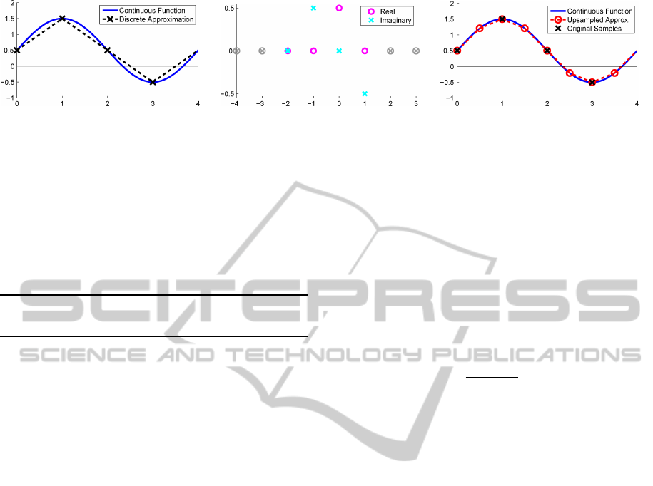
Figure 3: FFT-based upsampling process. Left: A periodic band-limited function with a period of 4, and its discrete ap-

proximation sampled at a frequency of 1. Middle: FFT coefﬁcients of the function in magenta and cyan. Because the input

function was real, the coefﬁcients have a Hermitian symmetry. The coefﬁcients are padded with zeros to the left and right,

corresponding to higher frequencies with an amplitude of zero. Right: The inverse FFT of the padded coefﬁcients results in

a higher-resolution approximation to the continuous function. Note that the even grid points of the upsampled approximation

agree with the original grid points.

Table 1: Root-mean-square interpolation errors for differ-

ent interpolation schemes in two turbulent ﬂow ﬁelds before

(orig) and after compression (comp), compared to the refer-

ence trigonometric interpolant. The interpolation error has

been evaluated in a grid of four times the original resolution.

Iso (range: 6.67) MHD (range: 2.77)

Interpolation orig comp orig comp

Lagrange8 0.86E-3 1.26E-3 3.48E-4 4.97E-4

Lagrange6 1.10E-3 1.60E-3 4.52E-4 6.32E-4

Lagrange4 1.71E-3 2.41E-3 7.20E-4 9.63E-4

Linear 5.15E-3 6.65E-3 2.29E-3 2.81E-3

the following, we ﬁrst introduce the error metrics we

use to analyze the accuracy of the computed trajecto-

ries.

4.1 Error Metrics

Due to errors induced by the employed interpolation

scheme and by lossy compression, a trajectory may

gradually diverge from the ground truth over time.

To evaluate the accuracy of computed trajectories,

an error metric is required to quantitatively measure

the difference between two trajectories starting at the

same seed point.

One obvious metric is the maximum or average

distance between trajectories s

(u), s

(u) along their

parameter u. In addition, several metrics exist which

measure some kind of distance between two curves,

such as the (discrete) Fr

echet distance (Eiter and

Mannila, 1994) and the distance under dynamic time

warping (DTW). While the Fr

echet distance corre-

sponds to a type of maximum distance, the DTW

distance is akin to an average distance. Both disre-

gard the u parametrization and instead are concerned

only with the shape of the curves. All these metrics

measure the distance along the complete trajectories.

However, once two particles have diverged by some

critical distance, their further behavior depends only

on the characteristics of the ﬂow ﬁeld: They might

diverge further or even converge again, but this pro-

vides no insight into the accuracy of the trajectory

computation. Therefore, we introduce a new metric

taking this into account, which we call the (clamped)

divergence rate. Instead of measuring a distance be-

tween trajectories, it computes the rate at which they

diverge. Given two trajectories s

(u), s

(u) over a pa-

rameter interval [u

, u

max

], we deﬁne their divergence

rate as

dist(u

div

)

div

− u

, where

dist(u) := ks

(u) − s

(u)k and

div

:= max



u ∈ [u

, u

max

]



∀ ˜u ∈ [u

, u] : dist( ˜u) ≤ ∆s



div

is the last point along the trajectories at which

they have not yet diverged by more than ∆s. In the

following experiments, we have set the critical dis-

tance ∆s equal to the grid spacing.

Our deﬁnition of the trajectory divergence rate is

similar in spirit to the idea of the ﬁnite-size Lyapunov

exponent (FSLE) (Aurell et al., 1997). The FSLE

measures the time it takes for two particles, initially

separated only by an inﬁnitesimal ε, to diverge by

some given distance, usually speciﬁed as a multiple

of ε. A fundamental difference is that in our case

both trajectories start at exactly the same position, and

we measure their divergence as an absolute distance

rather than relative to their initial separation.

4.2 Error Analysis

To compare the accuracy of particle trajectories com-

puted in the original and compressed data sets, and

via different interpolation schemes, a reference solu-

tion is required to which the trajectories can be com-

pared. For the used turbulence data sets, trigonomet-

ric interpolation is known to be exact. Since evaluat-

ing the trigonometric interpolant during particle trac-

ing is impracticable, we have upsampled the data sets

to four times the original resolution (see Section 3.1)

as the ground truth. Particle trajectories traced in the

AnalyzingtheEffectofLossyCompressiononParticleTracesinTurbulentVectorFields

283

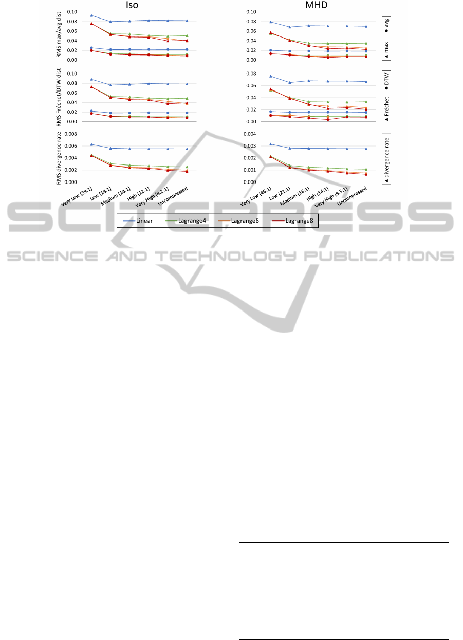
Figure 4: Accuracy of stream lines vs. compression quality using different interpolation schemes. Accuracy is reported as the

root mean square (RMS) of the individual trajectory distances (see Section 4.1), computed against trajectories traced using

the (approximate) trigonometric reference interpolation.

upsampled versions using 16th order Lagrange inter-

polation then act as the reference solution. While this

is not equivalent to true trigonometric interpolation

in the original data, the remaining error is expected

to be negligible since the difference between the two

times and four times upsampled versions is already

very small (cf. Section 3.1).

For the accuracy analysis of computed trajecto-

ries, we have generated a set of 4096 seed points in

each data set, that were randomly distributed over

the entire domain. Particles were traced from the

seed points through different versions of the data sets:

The upsampled reference version, the original un-

compressed data, and compressed versions at differ-

ent compression rates. The quantization steps for the

compressed versions were chosen equal to the errors

in linear and Lagrange4/6/8 interpolation as listed in

Table 1. In addition, we generated one high-quality

compressed version of each data set, where the quan-

tization step was set to half the Lagrange8 interpola-

tion error. The compressed ﬁle sizes and compression

rates (as the ratio of original size to compressed size)

are listed in Table 2.

To minimize the impact of inaccuracies due to nu-

merical integration errors, in all of our experiments

we used the Runge-Kutta method by (Dormand and

Prince, 1980). The method provides a 5th order so-

lution and a 4th order error estimate, which is used

for adaptive step size control. The error tolerance for

step size control was reduced until the accuracy of the

results did not improve any further.

Fig. 4 provides the main results of our accuracy

analysis. The graphs show the root mean square

(RMS) of the average, maximum, Frchet, and DTW

distance, as well as the divergence rate, over all tra-

jectories for different compression rates and interpo-

lation schemes. For reference, the grid spacing is

approximately 0.00614 in both data sets. The most

prominent ﬁnding is that linear interpolation performs

very poorly and eclipses the errors introduced at even

the highest compression rates. The differences be-

tween the other interpolation schemes are compar-

atively small; as expected, with some advantage of

the higher-order schemes. All distance metrics give

qualitatively similar results. However, all metrics ex-

cept for our novel divergence rate display a signiﬁ-

Table 2: File sizes and compression factors. For Very Low,

Low, Medium, and High, the quantization step was chosen

equal to the error in linear and Lagrange4/6/8 interpolation,

resp. (cf. Table 1); for Very High, to half the error in La-

grange8.

Iso MHD

Quality size factor size factor

Uncompressed 14.7 GB – 14.7 GB –

Very High 1.79 GB 8.21 1.55 GB 9.48

High 1.25 GB 11.8 1.06 GB 13.9

Medium 1.08 GB 13.6 942 MB 16.0

Low 843 MB 17.9 712 MB 21.1

Very Low 387 MB 38.9 331 MB 45.5

IVAPP2015-InternationalConferenceonInformationVisualizationTheoryandApplications

284

cant amount of noise in the results. This is caused

by a few individual trajectories with a very large dis-

tance to their reference. These trajectories have a very

large impact on the RMS distance, but actually carry

little information on the accuracy of the results, as ex-

plained in Section 4.1. The divergence rate, on the

other hand, handles such trajectories well.

The most important observation with regard to the

lossy compression is that when the quantization step

is chosen smaller than the interpolation error (e.g. La-

grange4 interpolation and a compression quality of

“Medium” or higher), the additional error introduced

by the compression is extremely small. For example,

switching from Lagrange6 to Lagrange4 interpolation

has a larger impact on the accuracy than switching

from uncompressed data to the “High” compression

quality in both data sets.

5 PARTICLE TRACING SYSTEM

We have integrated the presented compression layer

into an out-of-core GPU particle tracing system to fa-

cilitates an interactive visual exploration of large scale

turbulence ﬁelds on commodity PC hardware. In the

following we will ﬁrst give a brief system overview.

Next, we will evaluate its performance and, ﬁnally,

we will compare its performance to previous systems

that have employed large compute clusters to extract

integral lines from large scale (unsteady) ﬂow ﬁelds.

5.1 System

Our proposed system for out-of-core particle tracing

takes as input a sequence of 3D velocity ﬁelds, each

ﬁeld representing the state of a ﬂow ﬁeld at a different

point in time. We assume that the values in each ﬁeld

are given on a Cartesian grid. In a preprocess, each

grid is partitioned into a set of equally-sized bricks. A

halo region is added around each brick to allow proper

interpolation at brick boundaries. The bricks are com-

pressed before being stored sequentially on disk.

At runtime, the computation of particle trajecto-

ries is performed on the GPU. For that, bricks which

are required to perform the numerical integration are

requested from the CPU and cached in their com-

pressed form in main memory. The compression

reduces disk bandwidth requirements and allows us

to cache a large number of bricks. For use on the

GPU, the compressed brick data is uploaded into GPU

memory and immediately decompressed. In the cur-

rent implementation we use bricks of size 128

each

(including a halo region of size 4). We have found

that this size provides the best trade-off between lo-

cality of access and storage overhead for the halo

regions. Multiple bricks are stored in a brick atlas

whose size is chosen based on the amount of avail-

able GPU memory.

Fluid particles are advected in parallel on the GPU

to exploit memory bandwidth and computational ca-

pacities. We use the CUDA programming API and is-

sue one thread per particle, grouped into thread blocks

of size 128. Each thread advects the position of its

particle while the required ﬂow data is available in the

brick atlas. Since the set of bricks which are required

to perform the computation of all trajectories does not

ﬁt into GPU memory in general, only a subset can be

made available at a time. An additional index buffer

stores the mapping from a brick index (a tuple con-

sisting of a spatial index and an id for the time step)

to position in the brick atlas. If a particle enters a re-

gion for which the respective brick is missing in the

brick atlas (ﬂagged by a −1 in the index buffer), the

GPU requests this brick for the next round of trac-

ing. This is realized by atomically incrementing the

corresponding entry in an additionally requests buffer

which maps spatial regions and point in time to brick

indices.

The GPU stops when all particles a) must stop

because they are waiting for a brick to be uploaded

to the GPU, b) have been advected for a predeﬁned

amount of time, or c) have been advanced by a ﬁxed

maximum number of steps (64 in the current imple-

mentation). The CPU then downloads the requests

buffer and determines the bricks to be uploaded next

into the atlas–prioritized by their respective request

count. When path lines are traced, requested bricks

corresponding to an earlier time step are prioritized

higher so that all path lines advance in time at roughly

the same speed, thus reducing multiple uploads of the

same data during the execution of one multi-pass ad-

vection step. If the systems main memory is too small

to hold all necessary bricks, the CPU fetches the brick

data from disk and replaces an existing brick in mem-

ory based on an LRU (Least Recently Used) caching

strategy. The CPU also tracks the earliest time step

which was requested globally and pages out all brick

time steps older than that, since they will not be vis-

ited again by the current particles. The requested

bricks are then sent to the GPU and particle tracing

is restarted. The process is ﬁnished once all particles

have either reached their maximum age or left the do-

main.

Special care has to be taken whenever a parti-

cle moves close to a brick boundary. In this case it

has to be ensured that all velocity values required in

the integration step are available in the current brick.

AnalyzingtheEffectofLossyCompressiononParticleTracesinTurbulentVectorFields

285

While we employ a halo region to ensure that all val-

ues required by the support of the interpolation kernel

are available, for a multi-stage integration method not

only the initial particle location, but also all interme-

diate stages of the integrator must reside within the

admissible area. This can be guaranteed by adapting

the maximum integration step size ∆t appropriately.

5.2 Performance Evaluation

The performance of any particle tracing system de-

pends on a multitude of factors, such as the charac-

teristics of the data set, the number and placement

of seeding locations, and the total integration time.

This makes an exhaustive performance evaluation and

comparison to other approaches fairly difﬁcult. In-

stead, we tried to capture the typical performance

characteristics of our system. For both data sets, we

investigated the following two scenarios:

1. Sparse. This is the same scenario that was used

for pursuing the accuracy analysis. 4096 seeding

locations are distributed uniformly in the domain,

and particles are traced for 2.5 and 5 time units in

Iso and MHD, respectively.

2. Dense. This scenario models an interactive explo-

ration. 1024 seed points are placed within a small

box with an edge length of 10% of the domain

size. The particles are traced over 5 and 10 time

units in Iso and MHD, respectively.

All timings were measured on a PC with an Intel

Core i5-3570 CPU (quad-core, 3.4 GHz) with 8 GB

of DDR3-1600 RAM, equipped with an NVIDIA

GeForce GTX 680 GPU with 4 GB of video mem-

ory. The size of the brick atlas was set to 2 GB of

video memory.

We have traced particles starting from the se-

lected seed points in both the uncompressed and the

compressed data sets to demonstrate the performance

gains that can be achieved via compression. In all

experiments, Lagrange6 interpolation was performed;

the particle integration times are about 3× higher with

Lagrange8, and about 4× lower with Lagrange4 inter-

polation. When particle tracing was performed on the

compressed data, the timings refer to the “High” com-

pression quality. The decompression times for other

compression rates differ only very slightly. To mea-

sure the impact of disk I/O, we have run every bench-

mark a second time, so that all required data was al-

ready cached in CPU memory. With uncompressed

data, however, this was only possible for the dense

scenario; in case of sparse particle seeding, the size

of the working set exceeded the available CPU mem-

ory (even for stream lines extracted from a single time

step). Table 3 lists the time required for running each

scenario, and Table 4 lists the sizes of the correspond-

ing working sets.

It can be seen that the use of compression allows

us to trace thousands of characteristic lines within

seconds in the dense seeding scenario. In the sparse

seeding case, the required time is around an order of

magnitude higher. The reason becomes clear when

looking at the size of the working sets, which are

larger by roughly the same factor in those cases.

Without compression, the overall system perfor-

mance is clearly limited by disk bandwidth. In par-

ticular, in the sparse scenario, the working set was

so much larger than main memory (cf. Table 4)

that some bricks had to be loaded from disk multi-

ple times. Even when all required data is already

cached in CPU memory (which was only possible

in the dense scenario), the performance of the com-

pressed and uncompressed cases is very similar—the

runtime overhead caused by the additional decom-

pression step is very minor.

It is clear that when tracing path lines, the work-

ing sets are much larger because often many differ-

ent time steps of the same spatial brick are required.

In particular, the temporal distance between succes-

sive time steps is extremely small in both data sets

(0.002 time units for Iso, 0.0025 for MHD). Because

of this, the time required for path line computation is

spent almost exclusively on disk-to-CPU data trans-

fer and GPU decompression, and only a negligible

amount of time is spent on the actual particle integra-

tion (less than 1% in our tests). For example, tracing a

set of path lines with the dense seeding conﬁguration

through Iso takes about 6 minutes, with a working set

size of over 25 GB of compressed data. In the un-

compressed setting, the working set comprises over

300 GB. Correspondingly, tracing these path lines in

Table 3: Times in seconds for computing stream lines, both

for the cached case (C) and the un-cached case including

disk access times (U). Individual times for uploading the

data to the GPU (Upl, including decompression), particle

integration (Int), and disk I/O (IO, overlapping Upl and Int)

are listed separately.

Scenario Quality U C Upl Int IO

Iso dense

High 2.3 1.4 0.8 0.6 1.9

Uncomp 18.6 1.3 0.7 0.6 17.8

Iso sparse

High 21.6 16.4 12.4 3.8 14.9

Uncomp 156.9 n/a 10.7 3.8 156.4

MHD dense

High 3.4 2.3 1.4 0.8 2.8

Uncomp 26.3 2.3 1.4 0.8 25.6

MHD sparse

High 19.9 16.2 11.8 4.2 13.6

Uncomp 139.7 n/a 10.4 4.2 138.8

IVAPP2015-InternationalConferenceonInformationVisualizationTheoryandApplications

286

Table 4: Working set sizes in both compressed (High) and

uncompressed (Uncomp) form. Also shown is the number

of bricks in the working set (#B) as well as the number of

brick uploads during particle integration (#U).

Scenario High Uncomp #B #U

Iso dense 165.9 MB 2155.5 MB 92 92

Iso sparse 1280.6 MB 15058.9 MB 728 1341

MHD dense 243.8 MB 3231.0 MB 138 155

MHD sparse 1095.5 MB 15066.5 MB 729 1298

the uncompressed data set takes almost an hour, and

most of that time is spent on disk I/O. In MHD, the

time required for path line tracing is similar; in all

cases, the time scales proportionally to the working

set size.

5.3 Comparison to Previous Work

To the best of our knowledge, all previous techniques

for particle tracing in very large ﬂow ﬁelds have em-

ployed large compute clusters. Pugmire et al. (Pug-

mire et al., 2009) have used 512 CPUs to trace 10K

stream lines in two steady ﬂow ﬁelds comprising 512

million grid cells each. They report wall times of 10

to 100 seconds. Camp et al. (Camp et al., 2011) later

improved those timings to a few seconds for tracing

thousands of stream lines on 128 cores. Nouanesen-

gsy et al. (Nouanesengsy et al., 2011) achieve timings

between 10 and 100 seconds using 4096 cores for the

computation of 256K stream lines in regular grids of

up to 1.67 billion grid points, but at the cost of an

expensive preprocess. Peterka et al. (Peterka et al.,

2011) report computation times of about 20 seconds

using 8192 cores for 128K stream lines in a 1024

steady ﬂow, and several minutes for 32K lines in a

2304 × 4096 × 4096 steady ﬂow. In contrast to all

other mentioned approaches, they have also addressed

large unsteady ﬂow ﬁelds. In a 1408 ×1080× 1100×

32 unsteady ﬂow, the processing time is several min-

utes for 16K path lines on 4096 cores.

While an exact performance comparison to our tech-

nique is not possible due to the different data sets

and interpolation/integration schemes used, an order-

of-magnitude comparison reveals that our method

achieves competitive timings to the previous ap-

proaches in many cases, particularly in dense seeding

scenarios, while making use of only a single desktop

PC.

All in all it can be said that due to the use of an

effective compression scheme, the performance of

particle tracing in extremely large ﬂow ﬁelds can

be improved signiﬁcantly. It is clear that due to the

immense working set that is required when computing

path lines, fully interactive rates cannot be achieved

in this case.

6 CONCLUSION

In this paper we have discussed the application of

lossy compression of large scale turbulent vector

ﬁelds in the context of particle tracing to overcome

bandwidth limitations and storage requirements. And

we have demonstrated how this compression layer can

be integrate into an out-of-core GPU particle tracer,

to facilitate an interactive visual exploration of tera

scale data sets on a desktop PC. This gives rise to

integrating the exploration process into a researchers

daily workﬂow as a means to validate hypotheses. In

a number of experiments we have demonstrated that

compared to interpolation errors in the reconstruc-

tion of the velocity ﬁeld, the compression errors do

not signiﬁcantly affect the accuracy of the computed

trajectories. In the statistical sense, the quality of

the computed trajectories remains in the same order.

A performance analysis indicates that such a system

achieves a throughput that is comparable to that of

previous systems running on high-performance archi-

tectures.

The most challenging future avenue of research

will be the investigation of the effect of lossy data

compression in scenarios other than turbulence re-

search. The question will be whether lossy data com-

pression can also be applied to other ﬂow ﬁelds with-

out unduly affecting the accuracy of the resulting tra-

jectories. The main difﬁculty is that for most ﬂow

ﬁelds a “correct” interpolation scheme is not avail-

able, so the interpolation error can not be estimated

accurately. However, different criteria might be found

to steer the compression quality, e.g. given conﬁdence

intervals for the velocity values.

ACKNOWLEDGEMENTS

The work was partly funded by the European Union

under the ERC Advanced Grant 291372: Safer-Vis -

Uncertainty Visualization for Reliable Data Discov-

ery. The authors want to thank Charles Meneveau

from Johns Hopkins University and Tobias Pfaffel-

moser from TUM for helpful discussions and con-

structive criticism.

AnalyzingtheEffectofLossyCompressiononParticleTracesinTurbulentVectorFields

287

REFERENCES

Aurell, E., Boffetta, G., Crisanti, A., Paladin, G., and Vulpi-

ani, A. (1997). Predictability in the large: an extension

of the concept of Lyapunov exponent. J. Physics A:

Mathematical and General, 30(1):1–26.

Balachandar, S. and Maxey, M. R. (1989). Methods for

evaluating ﬂuid velocities in spectral simulations of

turbulence. J. Computational Physics, 83(1):96–125.

Balsa Rodriguez, M., Gobbetti, E., Iglesias Guiti

an, J.,

Makhinya, M., Marton, F., Pajarola, R., and Suter,

S. (2013). A survey of compressed GPU-based di-

rect volume rendering. In Eurographics 2013 - STARs,

pages 117–136.

Bruckschen, R., Kuester, F., Hamann, B., and Joy, K. I.

(2001). Real-time out-of-core visualization of parti-

cle traces. In Proc. IEEE 2001 Symp. on Parallel and

Large-Data Visualization and Graphics, pages 45–50.

Camp, D., Garth, C., Childs, H., Pugmire, D., and Joy, K.

(2011). Streamline integration using MPI-hybrid par-

allelism on a large multicore architecture. IEEE Trans.

Vis. Comput. Graphics, 17(11):1702–1713.

Dormand, J. R. and Prince, P. J. (1980). A family of em-

bedded Runge-Kutta formulae. J. Computational and

Applied Mathematics, 6(1):19–26.

Eiter, T. and Mannila, H. (1994). Computing discrete

echet distance. Technical Report CD-TR 94/64,

Technische Universit

at Wien.

Ellsworth, D., Green, B., and Moran, P. (2004). Interactive

terascale particle visualization. In IEEE Visualization,

pages 353–360.

Fout, N. and Ma, K.-L. (2012). An adaptive prediction-

based approach to lossless compression of ﬂoating-

point volume data. IEEE Trans. Vis. Comput. Graph-

ics, 18(12):2295–2304.

Fout, N. and Ma, K.-L. (2013). Fuzzy volume rendering.

IEEE Trans. Vis. Comput. Graphics, 18(12):2335–

2344.

Frigo, M. and Johnson, S. G. (2005). The design and im-

plementation of FFTW3. Proc. IEEE, 93(2):216–231.

Isenburg, M., Lindstrom, P., and Snoeyink, J. (2005). Loss-

less compression of predicted ﬂoating-point geometry.

Computer Aided Design, 37(8):869–877.

Lane, D. A. (1994). UFAT—a particle tracer for time-

dependent ﬂow ﬁelds. In IEEE Visualization, pages

257–264.

Laramee, R. S., Hauser, H., Doleisch, H., Vrolijk, B., Post,

F. H., and Weiskopf, D. (2004). The state of the art

in ﬂow visualization: Dense and texture-based tech-

niques. Computer Graphics Forum, 23(2):203–221.

Li, Y., Perlman, E., Wan, M., Yang, Y., Meneveau, C.,

Burns, R., Chen, S., Szalay, A., and Eyink, G. (2008).

A public turbulence database cluster and applications

to study Lagrangian evolution of velocity increments

in turbulence. J. Turbulence, 9:N31.

Lindstrom, P. and Isenburg, M. (2006). Fast and efﬁcient

compression of ﬂoating-point data. IEEE Trans. Vis.

Comput. Graphics, 12(5):1245–1250.

McLoughlin, T., Laramee, R. S., Peikert, R., Post, F. H., and

Chen, M. (2010). Over two decades of integration-

based, geometric ﬂow visualization. Computer

Graphics Forum, 29(6):1807–1829.

Nouanesengsy, B., Lee, T.-Y., and Shen, H.-W. (2011).

Load-balanced parallel streamline generation on large

scale vector ﬁelds. IEEE Trans. Vis. Comput. Graph-

ics, 17(12):1785–1794.

Peterka, T., Ross, R., Nouanesengsy, B., Lee, T.-Y., Shen,

H.-W., Kendall, W., and Huang, J. (2011). A study

of parallel particle tracing for steady-state and time-

varying ﬂow ﬁelds. In Parallel Distributed Processing

Symposium (IPDPS), pages 580–591.

Post, F. H., Vrolijk, B., Hauser, H., Laramee, R. S., and

Doleisch, H. (2003). The state of the art in ﬂow visu-

alisation: Feature extraction and tracking. Computer

Graphics Forum, 22(4):775–792.

Pugmire, D., Childs, H., Garth, C., Ahern, S., and Weber,

G. H. (2009). Scalable computation of streamlines on

very large datasets. In Proc. Conf. on High Perfor-

mance Computing, Networking, Storage and Analysis,

pages 16:1–16:12.

Rovelstad, A. L., Handler, R. A., and Bernard, P. S. (1994).

The effect of interpolation errors on the Lagrangian

analysis of simulated turbulent channel ﬂow. J. Com-

putational Physics, 110(1):190–195.

Sayood, K. (2005). Introduction to Data Compression.

Morgan Kaufmann Publ. Inc., 3rd edition.

Teitzel, C., Grosso, R., and Ertl, T. (1997). Efﬁcient and

reliable integration methods for particle tracing in un-

steady ﬂows on discrete meshes. In Visualization in

Scientiﬁc Computing, pages 31–41.

Treib, M., B

urger, K., Reichl, F., Meneveau, C., Szalay,

A., and Westermann, R. (2012). Turbulence visual-

ization at the terascale on desktop PCs. IEEE Trans.

Vis. Comput. Graphics, 18(12):2169–2177.

Yeung, P. K. and Pope, S. B. (1988). An algorithm for

tracking ﬂuid particles in numerical simulations of

homogeneous turbulence. J. Computational Physics,

79(2):373–416.

Yu, H., Wang, C., and Ma, K.-L. (2007). Parallel hierar-

chical visualization of large time-varying 3D vector

ﬁelds. In Proc. ACM/IEEE Conf. on Supercomputing,

pages 24:1–24:12.

Zheng, Z., Xu, W., and Mueller, K. (2010). VDVR: Veri-

ﬁable volume visualization of projection-based data.

IEEE Trans. Vis. Comput. Graphics, 16(6):1515–

1524.

IVAPP2015-InternationalConferenceonInformationVisualizationTheoryandApplications

288