
CORE: A COnfusion REduction Algorithm for Keypoints Filtering
Emilien Royer, Thibault Lelore and Fr
´
ed
´
eric Bouchara
Universit
´
e de Toulon, CNRS, LSIS UMR 7296, 83957 La Garde, France
Keywords:
Keypoints Filtering, Computer Vision, Feature Matching, Kernel Density Estimator.
Abstract:
In computer vision, extracting keypoints and computing associated features is the first step for many applica-
tions such as object recognition, image indexation, super-resolution or stereo-vision. In many cases, in order
to achieve good results, pre or post-processing are almost mandatory steps. In this paper, we propose a generic
pre-filtering method for floating point based descriptors which address the confusion problem due to repetitive
patterns. We sort keypoints by their unicity without taking into account any visual element but the feature
vectors’s statistical properties thanks to a kernel density estimation approach. Even if highly reduced in num-
ber, results show that keypoints subsets extracted are still relevant and our algorithm can be combined with
classical post-processing methods.
1 INTRODUCTION
Over the last recent years, keypoint detection and fea-
ture computation have seen an increasing attention in
computer vision researches, partly thanks to the ongo-
ing developpment of robotic and need of efficient im-
age databases queries. As a major contribution we can
cite the SIFT (Lowe, 1999) descriptor by D. Lowe.
Based on oriented gradient histograms, it proved to
be very efficient (Mikolajczyk and Schmid, 2005) and
inspired many others such as ASIFT (Morel and Yu,
2009) and SURF (Bay et al., 2006). Nowadays it is
still used in modern applications and has even been
ported to GPU architectures (Wu, 2007). However,
its computation times are not suitable for real-time
applications and the rises of small embedded plat-
forms such as smartphones aspired to faster compu-
tation times and less memory consumption. Thus, in
2010 Calonder et al. introduced the BRIEF (Calonder
et al., 2010) descripor, leading the way to the binary
descriptors field which produced ORB (Rublee et al.,
2011), BRISK (Leutenegger et al., 2011), FREAK
(Ortiz, 2012), D-BRIEF (Trzcinski and Lepetit, 2012)
and state-of-the-art Bin-boost (T. Trzcinski and Lep-
etit, 2013). In this area, some descriptors propose
a way of improving keypoint selection. For exam-
ple, ORB orders the FAST (Rosten and Drummond,
2006) responses by a harris corner measure (Harris
and Stephens, 1988). With our contribution, we pro-
pose a solution to both generally improve the selec-
tion and to address a specific case that we are present-
ing in the next section.
Figure 1: Example from the Zurich Building Image
Database of repetitive patterns leading in ”good-false”
matches with the sift descriptor.
1.1 The Repetitive Patterns Problem
A frequent and troublesome problem easily encoun-
tered when trying to match pairs in different images
is the repetitive pattern case, as we can see in figure 1:
the exact same pattern is present in multiple occuren-
cies within the image. These visual features make
it highly responsive to saliency analysis, returning
numerous keypoints that have almost the same fea-
ture vectors, which results in high confusion during
matching phase. Usually, the mismatch problem is
handled from a given putative point correspondences
by different kinds of approaches. A first kind of meth-
ods is based on a robust statistic estimation such as
LMS (Least Median of Squares) or M-estimators. In
(Deriche et al., 1994) Deriche et al. applied the LMS
for the robust estimation of the fundamental matrix.
In a similar approach Torr et al (Torr and Murray,
1995) proposed a method for the estimation of both
561
Royer E., Lelore T. and Bouchara F..
CORE: A COnfusion REduction Algorithm for Keypoints Filtering.
DOI: 10.5220/0005309405610568
In Proceedings of the 10th International Conference on Computer Vision Theory and Applications (VISAPP-2015), pages 561-568
ISBN: 978-989-758-089-5
Copyright
c
2015 SCITEPRESS (Science and Technology Publications, Lda.)

the fundamental matrix and motion estimation. An-
other robust estimation methods can be found in the
literature such as the algorithms proposed by Ma et al
(Zhao et al., 2011; Ma et al., 2014).
Another kind of methods, known as resampling
methods, act by trying to get a minimum subset
of mismatch-free correspondence. Methods belong-
ing to this category are usually extensions of the
well known RANSAC (RANdom SAmple Consen-
sus) (Fischler and Bolles, 1981) such as MLESAC
(Torr and Zisserman, 2000) or SCRAMSAC (Sattler
et al., 2009). We can also cite (Pang et al., 2014) and
(Rabin et al., 2007).
Other algorithms are based on different ap-
proaches as the ICF (Identifying point correspon-
dences by Correspondence Function) proposed by Li
et al (Li and Hu, 2010).
Another way to consider the mismatch problem is to
filter out repetitive patterns in each image. Such a pri-
ori approaches may be combined with the previous
methods that are performed a posteriori from a given
putative point correspondences. When looking at the
literature, detecting repetitive pattern is a known is-
sue in several different applications although it is re-
puted to be difficult. Repetitive structures can be de-
tected through symmetry analysis (Loy and Eklundh,
2006; Lee et al., 2008; Liu et al., 2004) and despite
being mostly 2D analysis, recent propositions try to
take into account non-planar 3D repetitive elements
(Jiang et al., 2011; Pauly et al., 2008). Mortensen et
al. enrich the SIFT descriptor with information about
the image global context (Mortensen et al., 2005), in-
spired by shape contexts (Belongie et al., 2002). The
SERP (Mok et al., 2011) descriptor and the CAKE
(Martins et al., 2012) keypoint extractor both rely on
kernel density estimation (Parzen, 1962). The first
one uses mean-shift clustering on SURF descriptors,
whereas the second one builds a new keypoint extrac-
tor based on shannon’s definition of information. As
we’re about to see in the next section, our approach
does also rely on kernel density estimation but in a
different way.
In this paper we propose a new approach to cope
with the keypoints confusion problem. We don’t take
into account the keypoints visual properties since they
may vary with the type of extractor chosen, but in-
stead we analyse the statistics properties of their asso-
ciated feature vectors. We estimate a numerical value
that is associated to the confusion risk of a given fea-
ture vector between another vector in a different im-
age. With this criterion, we can then sort the key-
points from low confusion risk, to high confusion risk.
With the right threshold, we can thus decide which
points should be discarded and which ones should be
kept. The rest of the paper is organized as follow:
Section 2.1 will present an overwiew of our proposed
method. In section 2.2 we will explain the criterion
computation. Section 2.3 will address the problem of
threshold setting. Finally, Section 3.1 will detail our
experiments methodology and sections 3.2 and 4 will
respectively present results and conclusions.
Further in the text we will use the following nota-
tion: we let P
x
(y) be the probability Pr(x = y) that the
variable x is equal to the value y.
2 PROPOSED METHOD
2.1 Overview
Let I be the image resulting of the observation (with
a camera) of a specific scene. Let I
0
be (a potential)
another observation of the same scene in which
changes result from various transformations such as
perspective changes, light modifications, etc. In our
model, I is deterministic whereas I
0
is a potential
(not yet observed) different version of I and is hence
considered to be stochastic. Let now u
i, i∈{1,...,N}
be D-dimensional feature vectors computed on
N keypoints of I and let u
0
i, i∈{1,...,N}
, be their N
respective equivalents in I
0
. We assume that even if
descriptors try to be invariant as much as possible to
most transformations, each feature vector in image
I is subject to slight variations in image I
0
we can
assimilate as randomness. By doing so we consider
u
0
i
as random vectors and we shall define a criterion
associated to each keypoints of I that characterizes
the confusion risk, i.e. a value correlated to the
probability that in I
0
, a vector u
0
j, j6=i
is closer to u
i
than u
j
.
For each keypoint i of I we define C
i
, the criterion, as
the probability density that any other random u
0
j, j6=i
is equal to u
i
, i.e. P
u
0
j, j6=i
(u
i
). This density should
act as a criterion for separating relevant and high
confusion risk keypoints.
From this definition, we can write:
C
i
≡ P
u
0
j, j6=i
(u
i
) =
∑
j6=i
Pr(k = j,u = u
i
) (1)
=
∑
j6=i
P
k, k6=i
( j)P
u/ j
(u
i
) (2)
where P
k, k6=i
( j) denotes the probability of choos-
ing keypoint j and P
u/ j
(.) is the probability den-
sity function (PDF) of the feature vector given the
keypoint number. We simply assume P
k, k6=i
( j) =
1
N−1
(the N −1 keypoints are equiprobable) and we
VISAPP2015-InternationalConferenceonComputerVisionTheoryandApplications
562

note P
u/ j
(u) =
1
h
K
|
u−u
j
|
h
where K is a normalized
symmetric function and h is a smoothing parameter.
We thus obtain the estimation of C
i
by the classical
Parzen-Rosenblatt kernel density estimator (KDE):
C
i
=
1
h(N −1)
∑
j6=i
K
u
i
−u
j
h
!
(3)
The CORE algorithm (given in Algorithm 1) is
very straightforward and easy to implement.
Algorithm 1: CORE algorithm.
Data: I : image input
Data: p : probability confusion tolerated
Data: D : descriptor dimension
Data: σ : average variance of descriptor’s
feature vectors
Data: C
th
← findThreshold(p, σ, D) (b)
Result: χ : keypoint set returned
K ← keypoint set detected
U ← associated feature vectors
for u
i
∈U do
c
i
← KDE(u
i
, U ) (a)
end
for k
i
∈ K do
if c
i
< C
th
then
Add k
i
to χ
end
end
return χ
Steps (a) and (b) are explained in next subsections.
2.2 Criterion Computation
We suppose that the vectors variations causes are nu-
merous and are either from natural origins or can be
considered as such. Therefore, it makes sense to con-
sider this behavior to be Gaussian. With this assump-
tion we can define K as the classical Gaussian Kernel:
K(u) =
1
√
2π
exp(−
1
2
u
2
) (4)
From such a definition, h takes the meaning of a
standard deviation σ of which we further address the
setting in our experiments section.
Thus, the criterion formula is :
C
i
=
1
(N −1)σ
√
2π
∑
i6= j
exp(−
d(u
i
,u
j
)
2
2σ
2
) (5)
where d(u
i
,u
j
) =
p
ku
i
−u
j
k is the euclidean dis-
tance between vector u
i
and u
j
.
2.3 Thresholding
Again, a relevant value of the threshold C
th
to apply
on the C
i, i∈{1,...,N}
can be estimated by considering
the confusion problem with a probabilistic point of
view. With the notations of the previous section,
let u
i
and u
0
i
be the feature vectors computed on the
same keypoint i of two different versions of a scene.
Let now v
i
= u
0
i
−u
i
, v
j
= u
0
j
−u
i
, d
2
i
= kv
i
k
2
and
d
2
j
= kv
j
k
2
where u
j
, u
0
j
are the corresponding feature
vectors computed on another keypoint j.
To estimate C
th
we shall express C
i
as a func-
tion of p = Pr(d
2
j
< d
2
i
) the probability of a confu-
sion. In our approach, p is a user-defined parame-
ter which tunes an acceptable confusion rate. To de-
rive this relation we need first to estimate P
d
2
j
(.), (and
hence P
v
j
(.) = P
u
0
j, j6=i
(.) −u
i
) which is governed by
the distribution of the u
j, j6=i
. However, we shall as-
sume that p only depends on the behavior of P
v
j
(.)
in a small neaborhood of u
i
. We hence approxi-
mate P
v
j
(.) by a D-dimensional uncorrelated Gaus-
sian distribution N(.; 0,Σ
v
j
) of which the central value
Pr(v
j
= 0) = P
v
j
(0) = C
i
by vertu of the definition of
C
i
given in the previous section. The diagonal element
σ
v
j
of the covariance matrix Σ
v
j
is simply related to C
i
by considering the normalisation condition on P
v
j
(.)
which can be written:
C
i
= (2πσ
2
v
j
)
−D/2
(6)
From this assumption, P
d
2
j
(.) is given by a chi-
squared distribution with D degres of freedom which
can be approximated by a Gaussian law N(.; E
j
,σ
j
)
due to the large value of D. The values of E
j
and σ
j
are classically related to the values of σ
v
j
and D by:
E
j
= σ
2
v
j
D and σ
j
= σ
2
v
j
√
2D.
Thanks to the Gaussian assumption on the u
0
i
val-
ues and using the same considerations as before,
we can also approximate P
d
2
i
by a gaussian law
N(.; E
i
,σ
i
) with E
i
= σ
2
D and σ
i
= σ
2
√
2D.
From these definitions we can now write:
p = Pr(d
2
j
< d
2
i
) (7)
=
Z
∞
−∞
Z
∞
x
P
d
2
j
(x)P
d
2
i
(y)dydx (8)
=
Z
∞
−∞
Z
∞
x
N(x; E
j
,σ
j
)N(y; E
i
,σ
i
)dydx (9)
CORE:ACOnfusionREductionAlgorithmforKeypointsFiltering
563
=
1
2
−
1
2σ
j
√
2π
Z
∞
−∞
exp
"
−(x −E
j
)
2
2σ
2
j
#
×
erf
x −E
i
σ
i
√
2
dx (10)
=
1
2
1 + erf
E
i
−E
j
q
2(σ
2
i
+ σ
2
j
)
(11)
After a straightforward, albeit a bit tedious, calcu-
lation we obtain from (11):
σ
2
v
j
= σ
2
D + 2
p
γ(D −γ)
D −2γ
(12)
with γ = 2 erf
−1
(2p −1)
2
(13)
From (12) and (13), the threshold C
th
which cor-
responds to a specific p is then given by (6).
3 EXPERIMENTS
3.1 Protocol
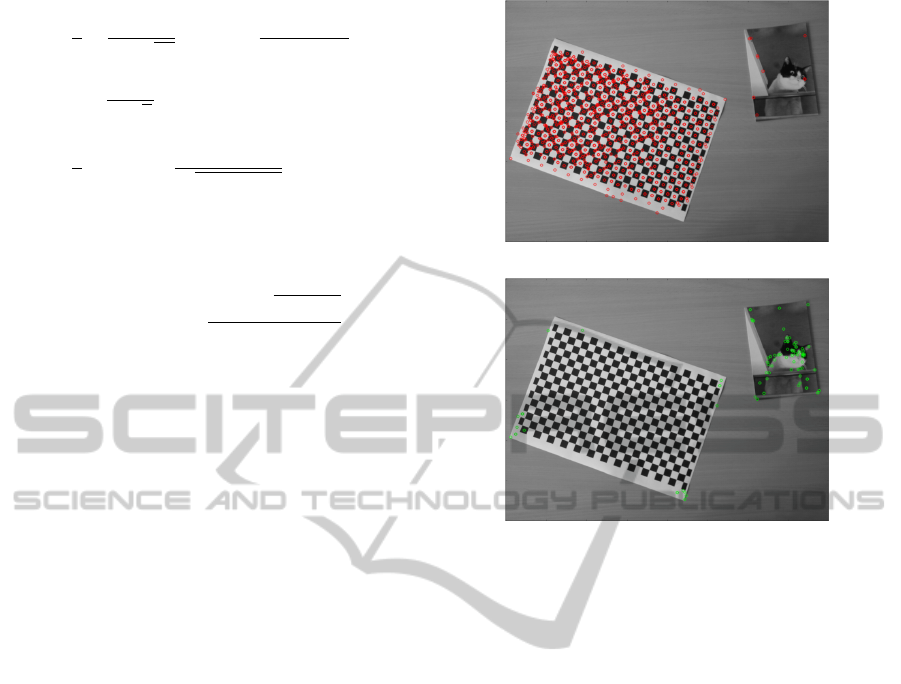
A quick example of keypoints filtered by proposed
method with the SIFT descriptor is shown with figure
2 where the confusion probability tolerated is 10%.
As we can see, the vast majority of the chessboard im-
age’s points are removed except for some on the cor-
ners, whereas the ones on the photograph are mostly
kept. This tends to confirm the wanted behavior of
our algorithm.
For validating our contribution, we’re looking to
prove that our algorithm does actually extract a bet-
ter keypoint subset less subject to confusion. For this,
we choose the classical application which consists in
matching keypoints pairs in different images. Specif-
icaly, we use a similar approach as used by SCRAM-
SAC by estimating an underlying model (i.e. funda-
mental matrix) and analysing the ratio of correspon-
dences consistent with it, called the inliers. We first
apply our experiments on a personnal set of 10 cou-
ples of document images captured by a smartphone
camera. Printed document images are very good can-
didates for confusion reduction due to the letters and
words repetitions. Moreover, their visual properties
make them highly responsive to saliency analysis, re-
sulting in a profusion of keypoints returned; usually
around 30.000 for a 2560x1920 picture with default
sift parameters. Thus, we also test our method as
a way of reducing huge keypoint sets without rely-
ing on visual analysis. As for the descriptor selec-
tion, considering its wide popularity and effiency, it
Figure 2: CORE application, top shows keypoints removed
and bottom is keypoints kept with p = 0.1.
is an obvious choice to base our protocol experiment
on the SIFT one. We also follow the idea of David
Lowe in (Lowe, 1999) to keep only high-quality fea-
ture matches: we reject poor matches by computing
the ratio between the best and second-best match (la-
belled 2NN for 2 nearest neighbours). If the ratio is
below a given threshold (we use 0.8), the match is
discarded as being low-quality.
We proceed as follows: for each image pair, we
apply our CORE algorithm on the keypoints returned
by SIFT. This returns a reduced keypoint set with
which we establish correspondences by brute-force
matching. We then use the RANSAC algorithm to
estimate the fundamental matrix and analyse the in-
lier ratio. For a fair comparison, we do the same with
another keypoint subset by following Lowe idea of
saliency analysis by a contrast threshold, so we end up
with a different keypoint set with equal size. On both
of these approaches, we also apply the SCRAMSAC
test to see how his matching filter behaves with these
two different pre-processing methods. Last, to serve
as a control test we extract a random keypoint subset
with same size in order to prove that our method (as
well as Lowe’s one) is better and makes more sense
than randomness. We repeat this for different p val-
ues, respectively 0.5, 0.25, 0.15, 0.10 and 0.05.
Finally, a valid criticism would be that analysing
the inlier ratio might not be always pertinent since the
VISAPP2015-InternationalConferenceonComputerVisionTheoryandApplications
564
fundamental matrix computed is not always accurate.
That’s why we propose a manual validation step: for
each couple of images, we apply the sift algorithm on
both images to detect and compute feature vectors.
From here, we build a first set of results by brute-
force matching the vectors; this will serve as a base
for comparisons. Thereafter, we apply the 2NN filter;
this is our second result-set. Last, we use our CORE
algorithm in order to remove keypoints that could lead
to confusion before applying the matching and previ-
ous filter, giving us our third and last result-set. For
each of these three sets, an operator manually evalu-
ates each match, giving us the table in the result sec-
tion 3.2. We also use the Zurich Image database (Shao
and Gool, 2003) instead of document images to show
that our algorithm is not exclusive to these and arbi-
trarly set a fixed p value of 0.1. Plus, since we’re not
computing average results here we also include two
image couples from images figure 2.
But before presenting our results, we still need to
address the σ setting as shown earlier in section 2.2:
since it characterizes the feature vector values varia-
tions, we use our images set to compute the global
mean value of variances of vectors elements thanks
to the correct matches manually checked. We found
it to be roughly around 32.135 for the SIFT descrip-
tor. However, even if early tests didn’t find notable
sensibility for values above 10, for very specific ap-
plications it could be understandable to re-evaluate it
more precisely.
3.2 Results
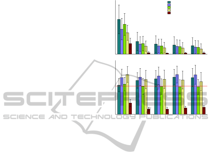
Results from first part of the experiment are presented
with figure 3. We see that for every p values, num-
ber of inliers is always greater than other subsets of
equal size resulting from saliency analysis. More-
over, with small p values (between 0.25 and 0.05), in-
lier ratio is always improved by CORE pre-processing
and starting with p = 0.15, CORE is doing better than
SCRAMSAC.
However, for p = 0.5 (50% of confusion toler-
ated), the inlier ratio is actually smaller with our
method. This could comes from the large confu-
sion tolerated that doesn’t remove enough keypoints:
we don’t take advantage of confusion reduction and
some very similar keypoints where removed whereas
their feature vector transformation may have not been
enough to generate confusion. So we recommend us-
ing p values being inferior than 0.25 and best results
seem to be achieved with 0.10. Not studied here, an-
other advantage of our algorithm would be the speed-
up gained during matching phase and model estima-
tion as we observed the average computation time to
50% 25% 15% 10% 5%
0
100
200
300
400
500
600
Percent of allowed confusion
# inliers
CORE filtered points
CORE filtered points + SCRAMSAC
Best SIFT points
Best SIFT points + SCRAMSAC
Randomly selected SIFT points
50% 25% 15% 10% 5%
0
0.1
0.2
0.3
0.4
0.5
0.6
0.7
Percent of allowed confusion
inlier ratio
Figure 3: Average results of first part of the test with differ-
ents filters. For each p value, we compare the results with
subsets of equal size. Top: raw numbers of inliers, bottom:
inlier ratio. Horizontal red line corresponds to SIFT inlier
ratio without any filtering.
be 20 times faster than without filtering. Finally, it
is worth noting that our pre-processing filter (CORE)
behaves well with post-processing (SCRAMSAC) by
always increasing the inlier ratio, regardless of the p
value used and the poor results from control test based
on randomness prove the relevance of pre-processing.
Now, concerning the second part of the test,
shown by table 1, we can see that our contribution
globally improves the good matching ratio: we find
a mean increasing value of 8.52% for the Zurich im-
ages. Images 4.c and 4.i show slight improvements
(with respectively 1.13% and 2.72% ratio increasing)
while the other ones extracted from this dataset range
from 6.22% to 13.8%. An explanation could come
from contextual information from the scene that could
prevent some confusion. The chessboard images that
hardly benefit from contextual information at all and
contain real repetition jump with respectively 36.99%
and 50.46%.
4 CONCLUSIONS
We presented the CORE algorithm, a pre-processing
filter which extract from a feature vector set a smaller
subset less subject to confusion by removing highly
CORE:ACOnfusionREductionAlgorithmforKeypointsFiltering
565
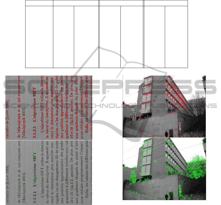
Table 1: Comparisons of the results (percentage, number of good matches/total matches) for three different approaches: first
column plain matching SIFT, second column SIFT with the 2NN filter (d = 0.8) and last column SIFT with both CORE
(p = 0.1) and 2NN filter (d = 0.8).
couple unfiltered 2NN CORE + 2NN
object0014 23.89% 322 / 1348 70.68% 258 / 365 81.82% 153 / 187
object0008 20.00% 336 / 1680 52.71% 204 / 387 66.51% 143 / 215
object0039 26.78% 448 / 1673 66.24% 310 / 468 67.37% 159 / 236
object0110 24.58% 222 / 903 57.29% 165 / 288 69.34% 95 / 137
object0164 25.16% 685 / 2723 65.66% 545 / 830 71.88% 317 / 441
object0170 41.61% 928 / 2230 80.25% 760 / 947 87.83% 469 / 534
object0181 32.35% 645 / 1994 74.77% 495 / 662 81.69% 290 / 355
object0192 18.75% 486 / 2592 64.78% 309 / 477 73.93% 241 / 326
object0106 25.06% 505 / 2015 74.71% 325 / 435 77.42% 216 / 279
chess01 15.92% 225 / 1413 47.49% 142 / 299 84.48% 49 / 58
chess02 10.72% 182 / 1698 35.98% 127 / 353 86.44% 51 / 59
Figure 4: Example from our personnal image document
dataset, top is keypoints removed and bottom is keypoints
kept. p = 0.1.
similar keypoints thanks to a probability approach.
Results showed that subsets extracted are more dis-
criminant and our approach can be combined with
post-processing ones.
However, due to the kernel density estimator used,
our algorithm can only be applied on floating point
based descriptors, putting aside the recent develop-
ments in the binary descriptors field. A binary ver-
sion of CORE will require a very different approach
and this will be the subject of future work.
Figure 5: Example from Zurich dataset, top is keypoints
removed and bottom is keypoints kept. p = 0.1.
ACKNOWLEDGEMENTS
This work was financially supported by the French re-
gion Provence-Alpes-C
ˆ
ote d’Azur (PACA).
REFERENCES
Bay, H., Tuytelaars, T., and Gool, L. (2006). Surf: Speeded
up robust features. In Computer Vision ECCV 2006,
VISAPP2015-InternationalConferenceonComputerVisionTheoryandApplications
566

volume 3951 of Lecture Notes in Computer Science,
pages 404–417. Springer Berlin Heidelberg.
Belongie, S., Malik, J., and Puzicha, J. (2002). Shape
matching and object recognition using shape contexts.
IEEE Trans. Pattern Anal. Mach. Intell., 24(4):509–
522.
Calonder, M., Lepetit, V., Strecha, C., and Fua, P. (2010).
Brief: Binary robust independent elementary features.
In Computer Vision ECCV 2010, volume 6314 of
Lecture Notes in Computer Science, pages 778–792.
Springer Berlin Heidelberg.
Deriche, R., Zhang, Z., Luong, Q.-T., and Faugeras, O.
(1994). Robust recovery of the epipolar geometry
for an uncalibrated stereo rig. In Proceedings of the
Third European Conference on Computer Vision (Vol.
1), ECCV ’94, pages 567–576, Secaucus, NJ, USA.
Springer-Verlag New York, Inc.
Fischler, M. A. and Bolles, R. C. (1981). Random sample
consensus: A paradigm for model fitting with appli-
cations to image analysis and automated cartography.
Commun. ACM, 24(6):381–395.
Harris, C. and Stephens, M. (1988). A combined corner
and edge detector. In In Proc. of Fourth Alvey Vision
Conference, pages 147–151.
Jiang, N., Tan, P., and Cheong, L. F. (2011). Multi-view
repetitive structure detection. In ICCV, pages 535–
542. IEEE.
Lee, S., Collins, R., and Liu, Y. (2008). Rotation symme-
try group detection via frequency analysis of frieze-
expansions. In Proceedings of CVPR 2008.
Leutenegger, S., Chli, M., and Siegwart, R. Y. (2011).
Brisk: Binary robust invariant scalable keypoints. In
Proceedings of the 2011 International Conference on
Computer Vision, ICCV ’11, pages 2548–2555, Wash-
ington, DC, USA. IEEE Computer Society.
Li, X. and Hu, Z. (2010). Rejecting mismatches by corre-
spondence function. Int. J. Comput. Vision, 89(1):1–
17.
Liu, Y., Collins, R., and Tsin, Y. (2004). A computational
model for periodic pattern perception based on frieze
and wallpaper groups. Pattern Analysis and Machine
Intelligence, IEEE Transactions on, 26(3):354–371.
Lowe, D. (1999). Object recognition from local scale-
invariant features. In Computer Vision, 1999. The Pro-
ceedings of the Seventh IEEE International Confer-
ence on, volume 2, pages 1150–1157 vol.2.
Loy, G. and Eklundh, J.-O. (2006). Detecting symmetry and
symmetric constellations of features. In Proceedings
of the 9th European Conference on Computer Vision
- Volume Part II, ECCV’06, pages 508–521, Berlin,
Heidelberg. Springer-Verlag.
Ma, J., Zhao, J., Tian, J., Yuille, A. L., and Tu, Z. (2014).
Robust point matching via vector field consensus.
IEEE Transactions on Image Processing, 23(4):1706–
1721.
Martins, P., Carvalho, P., and Gatta, C. (2012). Context
aware keypoint extraction for robust image represen-
tation. In Proceedings of the British Machine Vision
Conference, pages 100.1–100.12. BMVA Press.
Mikolajczyk, K. and Schmid, C. (2005). A perfor-
mance evaluation of local descriptors. Pattern Analy-
sis and Machine Intelligence, IEEE Transactions on,
27(10):1615–1630.
Mok, S. J., Jung, K., Ko, D. W., Lee, S. H., and Choi,
B.-U. (2011). Serp: Surf enhancer for repeated pat-
tern. In Proceedings of the 7th International Con-
ference on Advances in Visual Computing - Volume
Part II, ISVC’11, pages 578–587, Berlin, Heidelberg.
Springer-Verlag.
Morel, J.-M. and Yu, G. (2009). Asift: A new framework
for fully affine invariant image comparison. SIAM J.
Img. Sci., 2(2):438–469.
Mortensen, E. N., Deng, H., and Shapiro, L. (2005). A
sift descriptor with global context. In Proceedings
of the 2005 IEEE Computer Society Conference on
Computer Vision and Pattern Recognition (CVPR’05)
- Volume 1 - Volume 01, CVPR ’05, pages 184–190,
Washington, DC, USA. IEEE Computer Society.
Ortiz, R. (2012). Freak: Fast retina keypoint. In Proceed-
ings of the 2012 IEEE Conference on Computer Vision
and Pattern Recognition (CVPR), CVPR ’12, pages
510–517, Washington, DC, USA. IEEE Computer So-
ciety.
Pang, S., Xue, J., Tian, Q., and Zheng, N. (2014). Ex-
ploiting local linear geometric structure for identify-
ing correct matches. Computer Vision and Image Un-
derstanding, 128(0):51 – 64.
Parzen, E. (1962). On estimation of a probability den-
sity function and mode. The Annals of Mathematical
Statistics, 33(3):pp. 1065–1076.
Pauly, M., Mitra, N. J., Wallner, J., Pottmann, H., and
Guibas, L. J. (2008). Discovering structural regular-
ity in 3d geometry. In ACM SIGGRAPH 2008 Papers,
SIGGRAPH ’08, pages 43:1–43:11, New York, NY,
USA. ACM.
Rabin, J., Gousseau, Y., and Delon, J. (2007). A contrario
matching of local descriptors.
Rosten, E. and Drummond, T. (2006). Machine learning for
high-speed corner detection. In European Conference
on Computer Vision, volume 1, pages 430–443.
Rublee, E., Rabaud, V., Konolige, K., and Bradski, G.
(2011). Orb: An efficient alternative to sift or surf. In
Proceedings of the 2011 International Conference on
Computer Vision, ICCV ’11, pages 2564–2571, Wash-
ington, DC, USA. IEEE Computer Society.
Sattler, T., Leibe, B., and Kobbelt, L. (2009). Scramsac: Im-
proving ransac’s efficiency with a spatial consistency
filter. In ICCV, pages 2090–2097. IEEE.
Shao, T. S. H. and Gool, L. V. (2003). Zubud-zurich build-
ings database for image based recognition, technical
report no. 260.
T. Trzcinski, M. C. and Lepetit, V. (2013). Learning Image
Descriptors with Boosting. submitted to IEEE Trans-
actions on Pattern Analysis and Machine Intelligence
(PAMI).
Torr, P. H. S. and Murray, D. W. (1995). Outlier detection
and motion segmentation. pages 432–443.
Torr, P. H. S. and Zisserman, A. (2000). Mlesac: A new
robust estimator with application to estimating image
geometry. Comput. Vis. Image Underst., 78(1):138–
156.
CORE:ACOnfusionREductionAlgorithmforKeypointsFiltering
567

Trzcinski, T. and Lepetit, V. (2012). Efficient Discrimina-
tive Projections for Compact Binary Descriptors. In
European Conference on Computer Vision.
Wu, C. (2007). SiftGPU: A GPU implementa-
tion of scale invariant feature transform (SIFT).
http://cs.unc.edu/ ccwu/siftgpu.
Zhao, J., Ma, J., Tian, J., Ma, J., and Zhang, D. (2011). A
robust method for vector field learning with applica-
tion to mismatch removing. In Computer Vision and
Pattern Recognition (CVPR), 2011 IEEE Conference
on, pages 2977–2984.
VISAPP2015-InternationalConferenceonComputerVisionTheoryandApplications
568
