Executing Bag of Distributed Tasks on Virtually Unlimited Cloud

Resources

Long Thai, Blesson Varghese and Adam Barker

School of Computer Science, University of St Andrews, Fife, U.K.

Keywords:

Cloud Computing, Bag of Distributed Tasks, Cost vs Performance Trade-off, Decentralised Execution.

Abstract:

Bag-of-Distributed-Tasks (BoDT) application is the collection of identical and independent tasks each of

which requires a piece of input data located around the world. As a result, Cloud computing offers an effective

way to execute BoT application as it not only consists of multiple geographically distributed data centres but

also allows a user to pay for what is actually used. In this paper, BoDT on the Cloud using virtually unlim-

ited cloud resources is investigated. To this end, a heuristic algorithm is proposed to ﬁnd an execution plan

that takes budget constraints into account. Compared with other approaches, for the same given budget, the

proposed algorithm is able to reduce the overall execution time up to 50%.

1 INTRODUCTION

Bag-of-Tasks (BoT) is the collection of identical and

independent tasks executed by the same application

in any order. Bag-of-Distributed-Tasks (BoDT) is a

subset of BoT in which each task requires data from

somewhere around the globe. The location where a

task is executed is essential for keeping the execution

time of the BoDT low, since data is transferred from

a geographically distributed location. It is ideal to as-

sign tasks to locations that would be in geographically

close proximity to the data.

The centralised approach for executing BoDT, in

which data from multiple locations are transferred and

executed at a single location, tends to be ineffective

since some data resides very far from the selected lo-

cation and takes a long time to be downloaded. An-

other approach is to group the tasks of the BoDT in

such a way that each group can be executed near the

location of the data. However, this approach requires

an infrastructure which is decentralised and globally

distributed. Cloud computing is ideally suited for

this since public cloud providers have multiple data

centres which are globally distributed. Furthermore,

since clouds are available on a pay-as-you-go basis,

it is cost effective as a user only pays for Virtual Ma-

chines (VMs) that are required.

Cloud computing can facilitate the execution of

BoDT, and at the same time introduce the challenge

of assigning tasks to VMs by considering the loca-

tion for processing each task, the user’s budget con-

straint, as well as the desired performance, i.e. exe-

cution time, for executing the task. In an ideal case,

it is expected that maximum performance is obtained

while minimising the costs.

In our previous paper (Thai et al., 2014b), we ap-

proached this problem by assuming limited resources

were available. However, as Cloud providers offer

virtually unlimited resources, the limit should be de-

termined based on the user’s budget constraint. In this

paper, we present our approach for executing BoDT

on the Cloud with virtually unlimited resources and

is only limited by a user speciﬁed budget constraint.

Compared with other approaches, with the same given

budget, our algorithm is able to reduce the overall ex-

ecution time up to 50%.

The contributions of this paper are i) a mathemat-

ical model of executing a BoDT application on the

Cloud with budget constraints, ii) a heuristic algo-

rithm which assigns tasks to Cloud resources based

on their geographical locations, and iii) an evaluation

comparing our approach with centralised and round

robin approaches.

The remainder of paper is structured as follow.

Section II presents the mathematical model of the

problem. Section III introduces the heuristic algo-

rithms producing an execution plan based on the

user’s budget constraint. Section IV evaluates the ap-

proach. Section V presents the related work. Finally,

this paper is concluded in section VI.

373

Thai L., Varghese B. and Barker A..

Executing Bag of Distributed Tasks on Virtually Unlimited Cloud Resources.

DOI: 10.5220/0005403303730380

In Proceedings of the 5th International Conference on Cloud Computing and Services Science (CLOSER-2015), pages 373-380

ISBN: 978-989-758-104-5

 2015 SCITEPRESS (Science and Technology Publications, Lda.)

2 PROBLEM MODELLING

Let L = {l

...l

} be the list of Cloud locations, i.e.

location of Cloud provider’s data centres, and V M =

{vm

...} be the list of Cloud VMs. For vm ∈ V M,

∈ L denotes the location in which vm is deployed.

Let V M

⊂ V M be the list of all VMs deployed at lo-

cation l ∈ L. The number of items in V M is not ﬁxed

since a user can initiate as many VMs as possible.

Let T = {t

...t

} be the list of tasks, and size

de-

note the size of a task. The time (in seconds) taken

to transfer data from a task’s location to a Cloud lo-

cation is denoted as trans

t,l

. Similarly, trans

t,vm

for

vm ∈ V M is the cost of moving t to vm (or to a loca-

tion on which vm in running; trans

t,vm

= trans

t,l

We assume that there is only one type of VM is used,

hence, the cost of processing one unit of data is iden-

tical and is denoted as comp.

The time taken to execute task t at vm is:

exec

t,vm

= exec

t,l

= (trans

t,vm

+ comp) × size

(1)

Let T

⊂ T be the list of tasks executed in vm ∈

V M. All tasks must be executed and is represented as

the following constraint:

[

vm∈V M

= T (2)

One task should not be executed in more than one

location expressed as an additional constraint:

∩ T

0 for i, j ∈ V M and i 6= j (3)

The execution time of all tasks on vm ∈ V M is:

exec

∑

t∈T

exec

t,vm

(4)

As it takes some times to create a VM, the over-

head associated with the start up of each VM denoted

as start

up. The execution time of vm ∈ V M to exe-

cute all tasks in T

is:

exec

= start up + exec

(5)

It should be noted that Equation 5 can only be ap-

plied if there are task(s) assign to a VM, i.e. T

Otherwise, it is unnecessary to create a VM, thus its

execution time is zero.

Assuming each VM is charged by hour, i.e. 3600

seconds, the number of charged time blocks is:

= d

exec

3600

e (6)

Equation 6 contains the ceiling function, which

means the execution time is rounded up to the near-

est hour in order to calculate the number of used time

blocks. In other words, a user has to pay for a full

hour even if only a fraction of the hour is used.

Let P = {T

...T

} be the execution plan,

whose each item is a group of tasks assigned to one

vm ∈ V M. Let V M

denote the list of VMs used by

execution plan P. Similarly, let L

be the list of loca-

tions where all VMs of plan P are deployed. More-

over, P

denotes the execution plan for location l ∈ L,

which means L

= {l} and V M

= V M

As all VMs are running in parallel, the execution

time of a plan is equal to slowest VM’s:

exec

= max

vm∈V M

exec

(7)

The total number of time blocks used is the sum

of the time blocks used by each VM, represented as:

∑

vm∈V M

(8)

The budget constraint is the amount of money that

a user is willing to pay for executing the BoDT. Even

though Cloud providers charge users for using com-

pute time on virtual machines and transferring data,

only the renting cost is considered as the amount of

downloaded is unchanged for any given problem, i.e.

regardless the execution plan, the same amount of

data is downloaded, thus the data transferring cost.

The budget constraint is mapped onto the number

of allowed time blocks tb

by dividing the budget to

the cost of one time block (this is possible, because

of the assumption that there is only one VM type).

Hence, the problem of maximising the performance

of executing a BoDT on the Cloud with a given bud-

get constraint is to ﬁnd an execution plan P in order

to minimise exec

while keeping tb

= tb

and satis-

fying constraints in Equations 2 and 3.

3 ALGORITHMS

As stated in the previous section, the optimal plan for

executing BoDT on the Cloud with budget constraint

can be found by solving the mathematical model.

However, solving the mathematical model can take

considerable amount of time since it involves consid-

ering multiple possibilities of assigning tasks to dif-

ferent VMs at multiple Cloud locations. In this sec-

tion, we propose an alternative approach which is a

heuristic algorithm for ﬁnding an executing plan for a

BoDT based on a user’s budget constraint.

3.1 Select Initial Number of VMs at

Each Location

The main idea of the approach presented in this pa-

per is to specify a set of VMs for each location, then

CLOSER2015-5thInternationalConferenceonCloudComputingandServicesScience

374

to reduce the number until the total number of VMs

across all locations is tb

In order to determine the initial number of VMs at

each location, we make an assumption that it is pos-

sible to limit each VM to be executing in one time

block, i.e. if a VM ﬁnishes its execution in more than

one time block, its tasks can be split and scheduled

onto two VMs. Then, the total number of time blocks

is equal to the total number of VMs across all loca-

tions. Thus, the constraint tb

also limits the total

number of VMs, each of which uses no more than

one time block. Hence, initially, the number of VMs

at each location, i.e. V M

for l ∈ L, can be set to tb

3.2 Find Execution Plan based on

Budget Constraint

Let P

be the plan in which tasks are assigned to their

nearest location, i.e. the location in which exec

t,l

minimum. Each item in P

represents the list of tasks

assigned to a location (not a VM).

Algorithm 1: Find Execution Plan based on Budget Con-

straint.

1: function FIND PLAN(tb

, P

,V M)

2: P ←

3: for l ∈ L

4: P

← ASSIGN(T

,V M

)

5: if tb

> tb

then

6: FAIL

7: end if

8: P ← P

9: end for

10: P ← REDUCE(P,

0, T RUE)

11: if tb

> tb

then

12: P ← REDUCE(P,

0, FALSE)

13: end if

14: if tb

> tb

then

15: FAIL

16: end if

17: P ← BALANCE(P)

18: return P

19: end function

Algorithm 1 ﬁnds a plan with minimum execution

time based on the budget constraint tb

. The nearest

plan P

and the initial list of virtual machines V M are

provided as input. The algorithm uses three functions,

namely ASSIGN, REDUCE and BALANCE.

First of all, the algorithm assigns tasks to VMs

deployed in their nearest locations (From Line 3 to

9). Line 5 checks if the number of used time block in

a location is more than the budget constraint. If that

is the case, then it is impossible to ﬁnd an execution

plan satisfying the given budget constraint.

Secondly, some VMs are removed by moving its

tasks to other ones until the budget constraint is sat-

isﬁed (From Line 10 to 13). The reassignment can

be performed between VMs in the same location or

across multiple locations. If after reducing, the num-

ber of VMs is still higher than tb

, it is impossible to

satisfy the budget constraint (Lines 14 and 15).

Finally, as the execution times between VMs are

different (for example, one VM can take longer to ﬁn-

ish than the other ones) it is necessary to balance out

the execution times between all VMs so that they can

ﬁnish at the same time, thus reduce the overall execu-

tion time (Line 17).

3.3 Assign Tasks to VMs

Algorithm 2 aims to evenly distributed tasks from T

to the set of receiving VMs.

Algorithm 2: Assign Tasks to VMs.

1: function ASSIGN(T

,V M

)

2: T

← T

sorted by −exec

t,l

for t ∈ T

3: for t ∈ T

4: V M

← V M

ﬁltered exec

+ exec

t,vm

≤

3600

5: if V M

0 then

6: FAIL

7: end if

8: V M

← V M

sorted by (trans

t,vm

, exec

)

for vm ∈ V M

9: V M

← argmin

vm∈V M

trans

t,vm

10: vm ← V M

[0]

11: T

← T

∪ {t}

12: end for

13: P

← {T

for vm ∈ V M

}

14: return P

15: end function

First of all, tasks are sorted in descending order

based on their execution times (Line 2). Then, for

each task, all the VMs which can execute it without

requiring more than one time block is selected (Line

4). If there is no VM selected, i.e. it will take more

than one time block if a task is assigned to any given

VMs, the function fails (Lines 5 and 6).

All the selected VMs are sorted based on the dis-

tance between VM’s location and the task’s location,

and by their current execution time (Lines 8). The

task is assigned to the ﬁrst VM in the sorted collec-

tion (Lines 10 and 11). In other words, Algorithm 2

tries to assign a task to the nearest VM with the lowest

execution time.

ExecutingBagofDistributedTasksonVirtuallyUnlimitedCloudResources

375

3.4 Reduce the Number of VMs

Algorithm 3 is used to reduce the number of VMs by

moving all tasks from one VM to others which are ei-

ther in the same or on different locations. It is a recur-

sive process which takes the current plan P

, and the

list of VMs which cannot be removed from the plan

Ign, and the boolean value indicating if the reducing

process is applied locally or globally is local.

Algorithm 3: Reduce VMs.

1: function REDUCE(P, Ign, is local)

2: vm ← argmin

vm∈V M

exec

3: if is local = T RUE then

4: V M

← V M

− vm

5: else

6: V M

← V M

− vm

7: end if

8: P

← ASSIGN(T

,V M

)

9: if tb

< tb

then

10: P ← P

11: else

12: Ign ← Ign ∪ {vm}

13: end if

14: if tb

= tb

or Ign = V M

then

15: return V M

for l ∈ L

16: else

17: return LOCAL REDUCE(P

, Ign)

18: end if

19: end function

First, a VM with lowest execution time is selected

(Line 2). Then the remaining VMs, which can be ei-

ther in the same (Line 4) or on different Cloud loca-

tion (Line 6), are selected as receiving VMs.

After that, all tasks from selected VM are reas-

signed to other VMs (Line 8) by reusing the Algo-

rithm 2. Notably, the receiving VMs are not empty

but already contain some tasks.

If the reassignment reduces the number of VMs

(Line 9), the current plan is updated (Line 10). Other-

wise, the selected VM is added into the ignore list Ign

(Line 12). If the total time block satisﬁes the given

constraint or all VMs are ignored (Line 14), the pro-

cess stops and returns the current plan (Line 14), oth-

erwise it continues (Line 17).

3.5 Balance Tasks between VMs

After the budget constraint is satisﬁed, the execution

times between VMs can be uneven, i.e. some VMs

can have higher execution times than the others. As

the execution time of the plan exec

is based on the

VM with highest execution time, it is necessary to

balance out execution time between them.

Algorithm 4: Balancing Algorithm.

1: function BALANCE(P)

2: vm ← argmin

vm∈V M

exec

3: T

← T

sorted by −exec

t,vm

4: for t ∈ T

5: V M

← (V M

−{vm}) sorted by trans

t,vm

6: vm

← NULL

7: for vm

∈ V M

8: if t is never in vm

then AND rtc

exec

t,c

< rtc

9: vm

← vm

10: BREAK

11: end if

12: end for

13: if vm

6= NULL then

14: BREAK

15: end if

16: end for

17: if vm

6= NULL then

18: T

← T

−t

19: T

← T

∪ {t}

20: P ← (P − {T

, T

}) ∪ {T

, T

}

21: go to 2

22: end if

23: return P

24: end function

Algorithm 4 is an iterative process which tries to

move tasks from a VM with highest execution time

(Line 2) to the nearest VM possible. There are two

conditions for selecting a receiving VM: the selected

task is never assigned to it and its execution time after

receiving the task is not higher than the current exe-

cution time of the giving VM (Line 8).

3.6 Dynamic Scheduling To Avoid Idle

Even though Algorithm 1 aims to build the plan in

which all VMs ﬁnish their execution nearly at the

same time, due to the instability of the network and

other unaccountable factors, e.g. service failure, it is

not unusual for one VM to ﬁnish before others. As

the cost of a full hour is already paid, it is necessary

to utilise the remaining time of the ﬁnished VMs in

order to reduce not only idle and unpaid time but also

the execution time of other VMs.

Let rt

be the actual running time of a VM.

Let e

and T

be the estimated remaining ex-

ecution time and remaining tasks of vm ∈ V M.

CLOSER2015-5thInternationalConferenceonCloudComputingandServicesScience

376

terminate time denote the time it take for a VM to be

shut down. Finally, thr

and thr

are two threshold

values indicating the required remaining execution

time and number of tasks. As unﬁnished VMs are still

running when the reassignment is being performed,

those thresholds aim to avoid reassigning tasks al-

ready executed by one VM to another. The idea of

dynamic rescheduling is to move T

of a VM to an-

other ﬁnished one while satisfying thr

and thr

order to reducing its e

In order to support dynamic scheduling, we add a

feature which monitors the execution of VMs, keeps

track of the remaining tasks and execution times, and

detects a VM which has just ﬁnished its execution.

Algorithm 5: Dynamic Reassignment.

1: function REASSIGN(vm)

2: if 3600 − rt

< terminate time then

3: FAIL

4: end if

5: V M

← {V M

− {vm}} sorted by −e

for

∈ V M

6: vm

← NULL

7: for vm

∈ V M

8: if e

≤ thr

AND T

≤ thr

then

9: vm

← vm

10: BREAK

11: end if

12: end for

13: if vm

= NULL then

14: FAIL

15: end if

16: T

← T

sorted by trans

t,vm

for t ∈ T

17: T ←

18: el ← 3600 − rt

−terminate time

19: for t ∈ T

20: exec

← exec

+ exec

t,vm

21: if exec

≥

−thr

OR exec

> el then

22: BREAK

23: end if

24: T ← T ∪ {t}

25: T

← T

− {t}

26: end for

27: T

← T

− T

28: T

m ← T

29: T IME OUT (vm, el)

30: end function

Algorithm 5 is invoked every time a VM that has

just ﬁnished its execution. First, it check whether

there is enough time in a ﬁnished VM to execute some

tasks (Line 2). This check ensures that the ﬁnished

VM is able to be terminated before using another time

block. Then, the VM which not only has the highest

remaining execution time but also satisﬁes thr

and

thr

is selected (Lines 5 to 15).

After that, some of the tasks are moved from the

selected VM to the ﬁnished one until some conditions

are met: i) the execution time of the ﬁnishes VM is

greater or equal half of the remaining execution time

of the giving one, or, ii) the ﬁnished VM will take

more than one time block to ﬁnish its execution if

more tasks are added (from Lines 16 to 26).

Notably, Algorithm 5 is invoked only one at a

time, i.e. if there are multiple VMs that have com-

pleted executing their tasks, only one of them is reas-

signed tasks while other VMs wait.

Finally, the timeout feature is added to prevent the

ﬁnished VM, which is just assigned some more tasks,

to use more than one time block. Basically, it takes

the VM and the allowed execution time as arguments

(Line 29), if the VM is still running when time out,

it is automatically terminated and the remaining tasks

are moved to another VM with lowest remaining exe-

cution time, i.e. the one that is likely to ﬁnish ﬁrst.

4 EXPERIMENTAL EVALUATION

4.1 Set-up

In order to evaluate our proposed approach, we de-

veloped a word count application in which each task

involved downloading and counting the number of

words in a ﬁle from a remote server. Those ﬁles were

located on PlanetLab (PL), a test-bed for distributed

computing experiments (Chun et al., 2003). We had

5700 ﬁles across 38 PL nodes and the total amount

of data for each experiment run was more than 12 gi-

gabytes. The VMs were deployed on eight Amazon

Web Service (AWS) regions.

Prior to the experiment, we ran the test with fewer

tasks in order to collect the computational cost, i.e.

comp, and communicational costs between all AWS

regions and PlanetLab Nodes (i.e. trans).

Based on our algorithm, at least four VMs were

required to execute all 5700 tasks. We then set tb

{4, 6, 8, 10, 12, 14, 16, 18, 20}, i.e. the number of time

block (or VMs) that we wanted to use. For each value

of tb

, we ran the execution three times to ﬁnd the

mean and standard deviation.

For comparison, we implemented two simple ap-

proaches for executing BoDT on the Cloud:

• Centralised approach: one cen-

tralised location was selected as l

argmin

l∈L

(

∑

t∈T

trans

t,l

∗ size

), i.e. the cost

of moving all tasks to this location is a minimum

ExecutingBagofDistributedTasksonVirtuallyUnlimitedCloudResources

377

when compared to other locations. This approach

was developed based on the centralised approach

introduced in our previous paper (Thai et al.,

2014b), however, instead of using only one

VM at the selected location, in this paper, the

number of VMs was equal to the one used by

our proposed approach. In other words, this

centralised approach enjoyed the same execution

parallelism as the proposed one.

• Round Robin approach: for this approach, all

Cloud locations was sorted in ascending order

based on their costs of moving all tasks to them.

This means the ﬁrst Cloud location was the one

selected by the centralised approach. After that,

VMs were added to each location in circular or-

der, e.g. the ﬁrst VM was added to the ﬁrst Cloud

location in the sorted list.

For both approaches, Algorithm 2 was used to

evenly distribute tasks to all VMs.

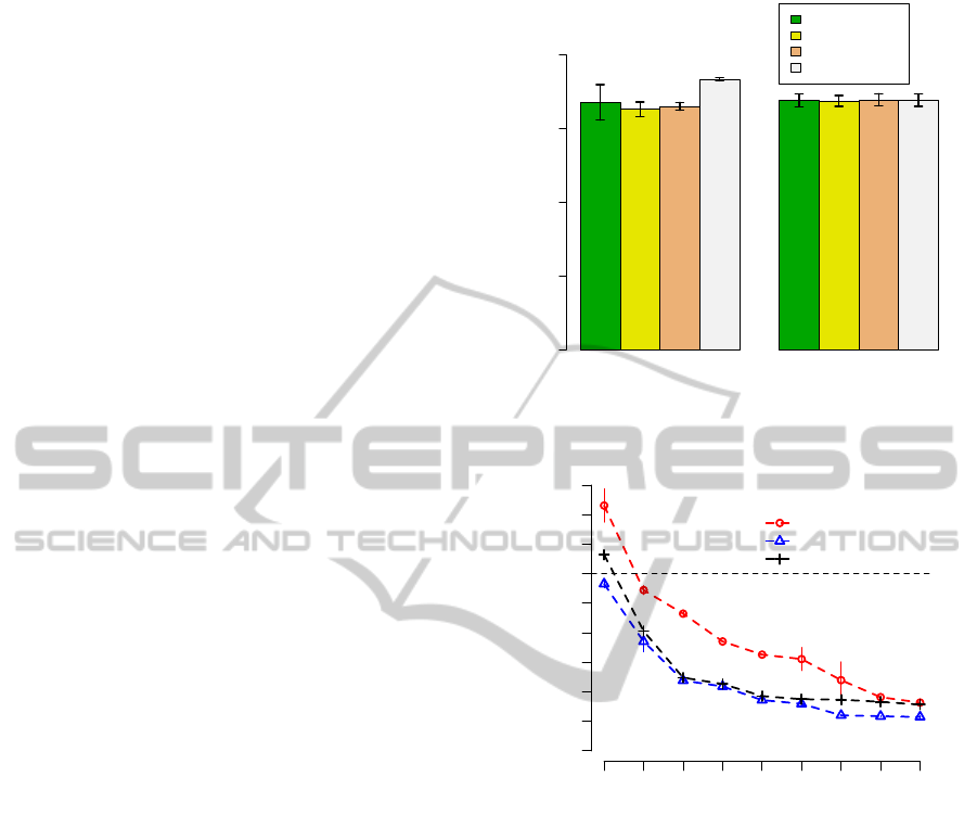
4.2 Dynamic Reassignment

Before going into the main experiment, it is neces-

sary to demonstrate the need of using dynamic reas-

signment for VMs that ﬁnish executing their assigned

tasks earlier than others. Figure 1 presents the result

of running the same execution plan with tb

= 4, i.e.

there were four VMs. Each bar represents the exe-

cution time of a VM. Without reassignment, one VM

took longer to ﬁnish its execution thus increasing the

overall execution time. Dynamic reassignment helped

to balance out the execution time between VMs so

that all VMs could ﬁnish at about the same time,

which in turn reduced the overall execution time. Dy-

namic reassignment is applied for the remaining ex-

periments presented in this section.

4.3 Experimental Results

Figure 2 presents the execution times corresponding

for each value of the number of VMs for all three ap-

proaches. The centralised approach had the highest

execution times as even though it selected the loca-

tion with lowest transfer cost for all tasks but some

tasks were very far from the Cloud location which re-

sulted in the high data transfer time. On the other

hand, the round robin approach performed better as

it deployed VMs at multiple Cloud locations, which

means it was possible for tasks to be executed near

their data sources. Finally, it is evident that for the

same number of VMs (or budget) our approach al-

ways had the lowest execution time in comparison

with other two.

Without_Reassignment With_Reassignment

Execution Time (seconds)

0 1000 2000 3000 4000

ap-southeast-1

ap-southeast-2

us-east-1

us-west-2

Figure 1: Compare execution without and with reassign-

ment.

Number of VMs

Execution Time (seconds)

4 6 8 10 12 14 16 18 20

0 600 1800 3000 4200 5400

Centralised

Decentralised

Round Robin

Figure 2: Execution Times.

A reason for the improvement is that our approach

not only deployed VMs at multiple locations but also

carefully selected those locations so that the major-

ity of tasks could be executed near their data sources.

The two simple approaches decided the location(s) of

VMs based on all tasks, by assuming all tasks were

assigned to one Cloud location. On the other hand,

our approach took a more ﬁne-grain method by as-

signing each task to its nearest location ﬁrst and then

reassigning them to others location until the budget

constraint was satisﬁed.

As the result, with the same given budget con-

straint, our approach was 30% to 50% faster than

the centralised approach. In comparison to the round

robin approach, ours was able to reduce the execution

times up to 30%.

Figure 3 presents the number of actual time

blocks, which can be mapped onto actual cost, con-

CLOSER2015-5thInternationalConferenceonCloudComputingandServicesScience

378

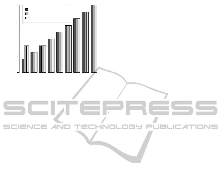
4 6 8 10 12 14 16 18 20

Number of VMs

Number of Time Blocks

0 5 10 15 20

Decentralised Approach

Centralised Approach

Round Robin Approach

Figure 3: Actual Number of Used Time Blocks, i.e. cost.

sumed by three approaches. It shows that our ap-

proach was able to satisfy the budget constraint in all

cases. Moreover, when there were four VMs, the cen-

tralised and round robin approaches were more ex-

pensive than the decentralised one. It was because

each of their VMs required more than one hour to ﬁn-

ish executing all the assigned tasks and the overall ex-

ecution time was higher than 3600 seconds, as shown

by Figure 2. Which means that the constraint tb

= 4

could only be satisﬁed by the decentralised approach.

4.4 Trade-off between Cost and

Performance

As presented in Figure 2, the higher the budget con-

straint is (i.e. more VMs), the better the performance

is. In theory, it is possible to keep adding more VMs

in order to achieve better performance. However, the

performance gain for each additional VM also de-

creases as the total number of VMs increases.

Hence, it is up the user to decide how much im-

provement in performance can be afforded. There

are some simple criteria to consider such as a deﬁned

budget constraint, the desired execution time or deﬁn-

ing a threshold in the performance gain (for example,

stop adding more VM(s) if the performance gain is

less than 60 seconds).

A user can also make the decision of how many

VMs to use based on the trade-off between perfor-

mance and cost, as mentioned in (Thai et al., 2014b).

5 RELATED WORK

In the Grid environment in which the resources are

shared between multiple organisations, the overall

performance of a distributed framework by process-

ing data in close proximity to where it resides is im-

proved (Ranganathan and Foster, 2002). Similarly, a

heuristic algorithm is proposed to improve the perfor-

mance of executing independent but ﬁle-sharing tasks

(Kaya and Aykanat, 2006). An auto-scaling algorithm

is proposed to satisfy deadline and budget constraints

when each task requires distributed data from multi-

ple sources (Venugopal and Buyya, 2005).

However, the application of Grid computing re-

search on Cloud computing is limited because: i)

the Cloud resources are (virtually) unlimited, hence

a user is free to add or remove VMs whenever she

wants but ii) the monetary cost factor has to be con-

sidered as the resource is not available free-of-charge.

Recently, running application on the Cloud has re-

ceived attention from many researchers. Statistical

learning had been used to schedule the execution of

BoT on the Cloud (Oprescu and Kielmann, 2010).

The method for scaling resource based on given bud-

get constraint and desired application performance

was also investigated (Mao et al., 2010). Neverthe-

less, those papers do not consider the location of data.

Cloud computing is employed for improving the

performance of data intensive application, such as

Hadoop, whose data is globally located (Ryden et al.,

2014). Research that takes geographical distance

into account while executing workﬂows is also re-

ported (Luckeneder and Barker, 2013; Thai et al.,

2014a). However, recent researches on applying

Cloud computing for applications with geographi-

cally distributed data only focus on improving the per-

formance without considering the monetary cost.

Our previous work (Thai et al., 2014b) aimed to

determine a plan for executing BoDT on the Cloud,

however, it made an assumption that there was only

one VM that could be deployed at each Cloud region.

Our paper differentiates itself from prior research

by taking advantage of the decentralised infrastruc-

ture of Cloud computing in executing BoDT applica-

tion. We tries to decide not only the amount of re-

sources but also the locations where resources, i.e.

VMs, must be located. Moreover, our research ex-

ploits of the virtually unlimited resources of Cloud

computing by letting a user decides how much re-

sources that she wants based on her budget. Fi-

nally, the trade-off between performance gain and ad-

ditional cost is also presented.

6 CONCLUSION

Due to its decentralised infrastructure and virtually

unlimited resources, Cloud computing is suitable to

ExecutingBagofDistributedTasksonVirtuallyUnlimitedCloudResources

379

execute BoDT, whose data is globally distributed all

over the world. It is challenging to decide how to as-

sign tasks to Cloud VMs based on a user’s budget con-

straint while minimising the execution time.

The above problem was mathematically modelled

in this paper. We also proposed a heuristic approach

which assigned BoDT to Cloud VM(s) in order to

maximise performance and to satisfy the allowed cost

provided by a user.

Furthermore, we implemented a dynamic reas-

signment feature to utilise the idle time of a VM

that completes execution ahead of others by assigning

tasks from other VMs onto it. This feature reduces the

overall execution time when a number of VMs take

longer to ﬁnish their execution due to service failure

or network instability.

Our approach was evaluated and able to provide

execution plans which satisﬁed given budget con-

straints. Compared to the centralised and round robin

approaches, our approach reduced the execution time

on average by 27%. Our approach was also able to

satisfy the low budget while the others did not.

In the future, we plan to further improve dynamic

resource provisioning and tasks scheduling so that

they can be performed during execution in order to

handle expected events, e.g. network instability or

machine failure. Moreover, the different types of

Cloud instances, which have varying performance and

cost will be taken into account.

ACKNOWLEDGEMENTS

This research is supported by the EPSRC grant

‘Working Together: Constraint Programming and

Cloud Computing’ (EP/K015745/1), a Royal Society

Industry Fellowship, an Impact Acceleration Account

Grant (IAA) and an Amazon Web Services (AWS)

Education Research Grant.

REFERENCES

Chun, B., Culler, D., Roscoe, T., Bavier, A., Peterson, L.,

Wawrzoniak, M., and Bowman, M. (2003). Planet-

lab: An overlay testbed for broad-coverage services.

SIGCOMM Comput. Commun. Rev., 33(3):3–12.

Kaya, K. and Aykanat, C. (2006). Iterative-improvement-

based heuristics for adaptive scheduling of tasks shar-

ing ﬁles on heterogeneous master-slave environments.

Parallel and Distributed Systems, IEEE Transactions

on, 17(8):883–896.

Luckeneder, M. and Barker, A. (2013). Location, location,

location: Data-intensive distributed computing in the

cloud. In In Proceedings of IEEE CloudCom 2013,

pages 647–653.

Mao, M., Li, J., and Humphrey, M. (2010). Cloud auto-

scaling with deadline and budget constraints. In Grid

Computing (GRID), 2010 11th IEEE/ACM Interna-

tional Conference on, pages 41–48.

Oprescu, A. and Kielmann, T. (2010). Bag-of-tasks

scheduling under budget constraints. In Cloud Com-

puting Technology and Science (CloudCom), 2010

IEEE Second International Conference on, pages

351–359.

Ranganathan, K. and Foster, I. (2002). Decoupling compu-

tation and data scheduling in distributed data-intensive

applications. In Proceedings of the 11th IEEE Interna-

tional Symposium on High Performance Distributed

Computing, HPDC ’02, pages 352–, Washington, DC,

USA. IEEE Computer Society.

Ryden, M., Oh, K., Chandra, A., and Weissman, J. B.

(2014). Nebula: Distributed edge cloud for data in-

tensive computing.

Thai, L., Barker, A., Varghese, B., Akgun, O., and Miguel,

I. (2014a). Optimal deployment of geographically dis-

tributed workﬂow engines on the cloud. In 6th IEEE

International Conference on Cloud Computing Tech-

nology and Science (CloudCom 2014).

Thai, L., Varghese, B., and Barker, A. (2014b). Execut-

ing bag of distributed tasks on the cloud: Investi-

gating the trade-offs between performance and cost.

In Cloud Computing Technology and Science (Cloud-

Com), 2014 IEEE 6th International Conference on,

pages 400–407.

Venugopal, S. and Buyya, R. (2005). A deadline and bud-

get constrained scheduling algorithm for escience ap-

plications on data grids. In in Proc. of 6th Inter-

national Conference on Algorithms and Architectures

for Parallel Processing (ICA3PP-2005, pages 60–72.

Springer-Verlag.

CLOSER2015-5thInternationalConferenceonCloudComputingandServicesScience

380