
Software Environments as Learning Tools for
Modeling Engineering Systems
A Case Study on Decentralized Multi-loop Control System
T. R. Melo
1
, L. C. Silva
2
, A. Perkusich
3
, J. J. Silva
3
and J. S. da Rocha Neto
3
1
Post-Graduate Program in Electrical Engineering - PPgEE - COPELE, Campina Grande - PB, Brazil
2
Embedded Systems and Computer Pervasive Laboratory (Embedded Lab), Campina Grande - PB, Brazil
3
Department of Electrical Engineering (DEE), Federal University of Campina Grande (UFCG), 58429-900, Campina
Grande - PB, Brazil
Keywords:
Simulation Models, Didactic Platform, Decentralized Multi-loop Control System, Simulink, Ptolemy.
Abstract:
This paper describes the usage of the Matlab/Simulink and Ptolemy II environments as learning tools in the
implementation of simulation models, which represent the decentralized multi-loop control system proposed
for a fouling detection didactic platform. The platform is treated as a two-input two-output (TITO) plant with
time delay, i.e., the voltage and current as the plant inputs and the flow and pressure as the plant outputs. In
both the software environments, the control system is modeled as a cyber-physical system (CPS). Constructive
details of each simulation model are shown, even as the main advantages and disadvantages of each learning
tool are discussed and evaluated by engineering students.
1 INTRODUCTION
In general, the engineering systems are characteri-
zed such as cyber-physical systems due to include
physics, computation, and networking aspects. These
systems require model combinations that integrate the
continuous dynamics of physical processes with the
discrete dynamics of computational platforms (Ptole-
maeus, 2014; Mosterman et al., 2012).
The modeling and simulating combinations of
discrete and continuous dynamics are still challeng-
ing (Lee, 2014). Nevertheless, the computation can
be identified as the main element that enables the de-
sign and analysis of the complex systems.
Among the software environments available, the
Matlab/Simulink
1
is a commercially tool suite used
to simulate control systems and also to generate and
verify embeddedcode, e.g., for prototyping. Simulink
defines a fixed model of computation that can only
be adapted to some extent by means of so-called
solvers as well as via the triggering of block exe-
cutions (Derler et al., 2008). The Ptolemy II
2
is
an open-source simulation environment based in Java
languagethat serves toexperimentdifferentmodels of
1
The MathWorks. Available from:
http://www.mathworks.com/products/simulink/
2
Ptolemy Project. Available from:
http://ptolemy.eecs.berkeley.edu/ptolemyII/
computation (MoCs), which are used to specify the
“laws of physics” that govern the concurrent execu-
tion and the interaction between computational com-
ponents (Ptolemaeus, 2014). Besides, the combina-
tion of MoCs allows to represent heterogeneous mo-
dels.
In this context, the goal in this work is to describe
the usage of the Matlab/Simulink and Ptolemy II en-
vironments as learning tools in the implementation of
simulation models, which represent the decentralized
multi-loop control system proposed for a fouling de-
tection didactic platform. The constructive details of
each simulation model are shown, even as the main
advantages and disadvantages of each learning tool
are discussed and evaluated by engineering students.
2 OVERVIEW ON MODELING
ENGINEERING SYSTEMS
Modeling is an important topic in engineering and
computation, which allows to represent and analyze
a physical problem from the construction of a model.
According to IEEE 610.12-1990 (IEEE, 1990), a
model is an approximation, representation, or ideali-
zation of selected aspects of the structure, behavior,
operation, or other characteristics of a real-world pro-
224
R. Melo T., C. Silva L., Perkusich A., J. Silva J. and S. Rocha Neto J..
Software Environments as Learning Tools for Modeling Engineering Systems - A Case Study on Decentralized Multi-loop Control System.
DOI: 10.5220/0005440402240231
In Proceedings of the 7th International Conference on Computer Supported Education (CSEDU-2015), pages 224-231
ISBN: 978-989-758-108-3
Copyright
c
2015 SCITEPRESS (Science and Technology Publications, Lda.)
cess, concept, or system, i.e., an abstraction. Depend-
ing of the physical problem in study, the models can
be obtained in continuous-time or discrete-time.
In the modeling of continuous behavior, the sys-
tem model may be represented by a ordinary diffe-
rential equation (ODE) or a set of integral equations,
which can be solved if initial and/or boundary condi-
tions were specified correctly.
The more informations are extracted of the engi-
neering system with continuous dynamics, more ac-
curately the model represents the physics. However,
the detailed modeling rarely helps in developing in-
sight about macroscopic system behavior and conse-
quently increased the simulation cost. Therefore, a
model with high fidelity has only this feature in some
regime of operation (Lee, 2014).
In the modeling of discrete behavior, the model
obtained is a state machine that each transition maps
the input valuations to the output valuations, depend-
ing on its current state. If the set of possible states is
finite, then the model is named as finite-state machine
(FSM) (Ptolemaeus, 2014). The FSMs are largely
used in control applications.
Due to the complexity of the engineering systems,
they present the continuous and discrete dynamics si-
multaneously, in which are known as hybrid systems.
From the area of computer simulation, the engi-
neering students can perform the analysis of hybrid
systems, in order to investigate relations and interac-
tions among components, to verify different solutions
and to test capabilities and technical characteristics of
the system (Despotovi-Zraki et al., 2014).
3 PLATFORM FOR FOULING
DETECTION
In order to understand the model-based systems engi-
neering obtained to control the fouling detection di-
dactic platform, the main features of the platform and
of the control system are presented.
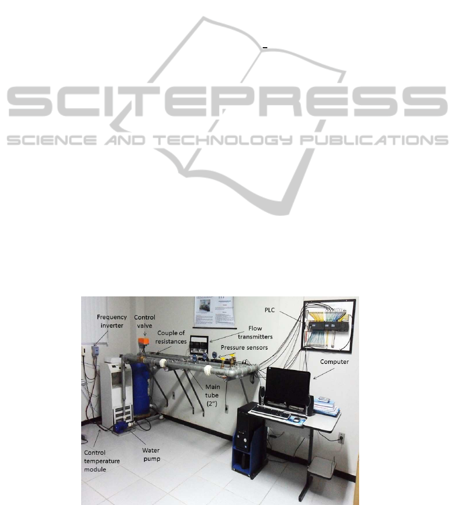
3.1 Physical Characteristics
The didactic platform shown in Fig. 1 is characterized
as a distributed monitoring of fluid transport system
with galvanized iron tubes of different diameters (1
inch, 1
1
2
inch and 2 inch) for the study of the fouling
phenomenon.
For the monitoring and control of this phe-
nomenon, on the didactic platform were used three
flow sensors and three pressure sensors, which were
fixed in each type of tube and one temperature sen-
sor which was submerged in the fluid (in this case,
the water) stored in a 100 liters tank. Besides, there
are one control valve with electric actuator and two
manual valves for outflow control, even as one fre-
quency inverter which is used for the rotate velocity
control of the water pump.
Furthermore, there is one PLC (Programmable
Logic Controller) responsible by the technology in-
tegration between sensors, actuators and computer
on the didactic platform. The sensors communicates
with the S7-200 PLC via 4-20 mA standard and the
actuators communicates with controller using the 4-
20 mA and 0-10 V standard.
Figure 1: Photograph of the fouling detection experimental platform.
SoftwareEnvironmentsasLearningToolsforModelingEngineeringSystems-ACaseStudyonDecentralizedMulti-loop
ControlSystem
225
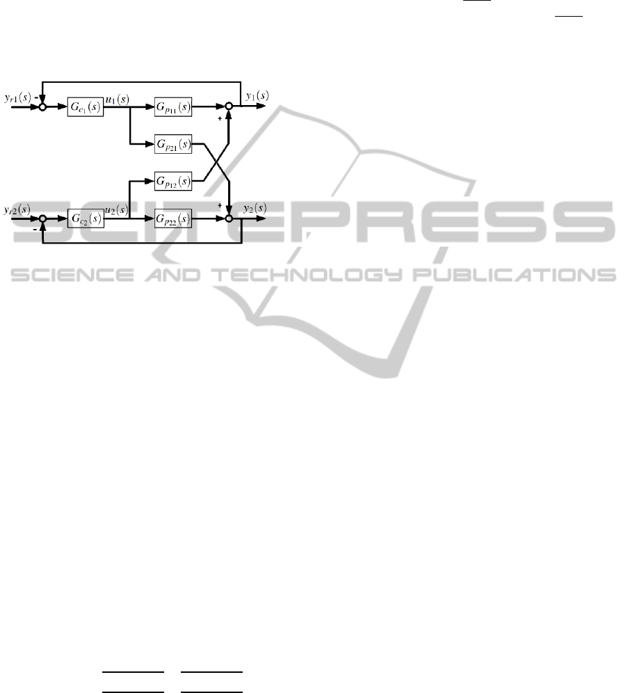
3.2 Control System Proposed
The decentralized control structure proposed for the
didactic platform, considering as a TITO plant, can be
observed in Fig. 2. Based in the relative normalized
gain array (RNGA) criteria (He et al., 2009), the loop
pairing chosen to control the didactic platform was
the off-diagonal pairing (1-2/2-1).
Figure 2: Block diagram of the decentralized control struc-
ture for a TITO plant.
In this control structure, the follow definitions
were done:
• The u
1
(s) and u
2
(s) represent the voltage signal
v(s) and the current signal i(s) applied on the ac-
tuators of the experimental platform, e.g., the fre-
quency inverter and the control valve;
• The y
1
(s) and y
2
(s) represent the flow measure
q(s) and the pressure measure p(s) monitored by
means of the flow and pressure sensors in the 2
inch tube;
• The y
r1
(s) and y
r2
(s) represent the reference flow
and the reference pressure which will be adopted
for operating in the 2 inch tube.
Thus, the transfer matrix G
p
(s) of the TITO plant
in study is a set of fisrt order plus dead time (FOPDT)
systems, according to Equation (1):
G
p
(s) =
G
p
11
(s) G
p
12
(s)
G
p
21
(s) G
p
22
(s)
⇒ G
p
(s) =
"
3.693e
−3.0021s
6.612s+1
1.956e
−3.0328s
21.26s+1
8.844e
−3.0021s
3.826s+1
3.026e
−3.0328s
19.17s+1
#
(1)
The transfer matrix G
c
(s), in Equation (2), has
compatible dimension with G
p
(s) and it is composed
by two PI decentralized controllers. Due to the off-
diagonal pairing, the controller G
c
1
(s) is applied to
control y
1
(s) by using u
2
(s) and the controller G
c
2
(s)
is applied to control y
2
(s) by using u
1
(s).
G
c
(s) =
G
c
1
(s) 0
0 G
c
2
(s)
⇒ G
c
(s) =
1.1891+
0.0562
s
0
0 0.0480+
0.0126
s
(2)
4 SIMULATION MODELS OF
THE DECENTRALIZED
CONTROL STRUCTURE
From the software environments chosen, the simula-
tion models of the decentralized control structure for
the didactic platform were implemented.
The complete description of each model is pre-
sented in the subsections 4.1 and 4.2.
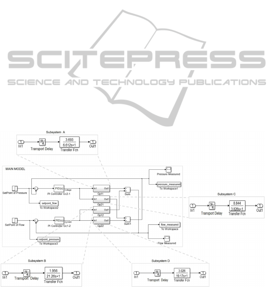
4.1 Modeling in Simulink
On the Simulink environment from The MathWorks,
the simulation model is implemented using hierar-
chical block diagram model based on the dataflow
paradigm. Each block is predefined in extensive and
expandable libraries for different types of models.
Besides, the blocks implementation is hidden in the
simulation engine.
When the model increases in size and complexity,
this can be simplified by grouping blocks into subsys-
tems, increasing the abstraction level of the model.
These subsystems must present the same dynamics
of the main model, which is in general a continuous
behavior.
To model the didactic platform as a TITO plant,
on the Simulink were created four subsystems named
as Gp11, Gp12, Gp21 and Gp22 to represent the
transfer functions that compose the transfer matrix
G
p
(s). Each subsystem is constituted by one-input
and one-output ports, which can be the input v(s) or
i(s), and the output q(s) or p(s), depending of the
transfer function. These ports are interconnected via
the blocks Transport Delay (which define the time de-
lay of the plant equals 3 seconds) and Transfer Fcn
(which specify the numerator and denominator coef-
ficients of the transfer function).
The PI decentralized controllers were obtained by
means of two blocks PID Controller named as Gc2−
1 (to control the pressure from the voltage signal) and
Gc1− 2 (to control the flow from the current signal).
The gains K
p
and K
i
of these controllers present the
same values obtained in Equation (2).
The set-point values of flow and pressure are de-
fined in each loop using the block Step. For the flow,
CSEDU2015-7thInternationalConferenceonComputerSupportedEducation
226

the set-point chosen was equals 18 LPM, and for the
pressure the value was equals 33 mBar.
The common outputs of the transfer functions
were added by means of two blocks Sum. Using the
same block, the negative feedback of the loops can be
implemented in off-diagonal paring.
At last, the flow and pressure curves along time
were observed using the block Scope. The values
are stored on the MATLAB console by means of the
block To Workspace.
4.2 Modeling in Ptolemy
On the Ptolemy II enviroment, the simulation model
to be implemented is based in hierarchical actor
model. The actors are components that execute con-
currently and share data with each other by sending
messages by means of input/output ports. All the
messages communicated via a port is referred to a sig-
nal. Besides, the connection between actors is esta-
blished by a relation (Ptolemaeus, 2014).
The director is a MoC which specifies the se-
mantic domain of the simulation. Furthermore, the
Ptolemy II allows to build submodels which use
others domains due to support heterogeneous model-
ing.
Relative to the modeling of the didactic platform
as a TITO plant, four ports were used to represent the
inputs v(s), i(s), and the outputs q(s), p(s). The trans-
fer matrix G
p
(s) was modeled using a opaque com-
posite actor (i.e., actor model that has not director)
named as DidacticPlatform, which is constituted by
four actors ContinuousTransferFunction (to symbol
the transfer functions G
p
11
(s), G
p
12
(s), G
p
21
(s) and
G
p
22
(s)) and two actors AddSubtract (to sum the com-
mon outputs of the transfer functions).
The control system were implemented using
modal models, where a multiplicity of distinct abs-
tract models are combined to model the same sys-
tem (Lee, 2014). Thus, the PI decentralized con-
trollers were obtained by means of two modal models
named as Controller21 (to control the pressure from
the voltage signal) and Controller12 (to control the
flow from the current signal). Each model is com-
posed by two control level, which are distinguished
by the domain.
In the high-level control, there is a discrete-time
model constituted by a FSM with two states associ-
ated to the dynamics imposed on actuator. For the
Controller21, the states are to increase or to decrease
the frequency on the frequency inverter; and for the
Controller12, the states are to open or to close the
control valve.
In the low-level control, there is continuous-time
model composed by a Continuous-Director and a set
of actors Gain, Integrator and AddSubtract intercon-
nected to execute the proportional-integrative action
of the controller. The gains K
p
and K
i
of the Con-
troller12 and Controller21 models present the same
values obtained for the controllers G
c
1
(s) and G
c
2
(s),
respectively.
The connection between the control levels were
realized by means of the states refinements. Each re-
finement specifies a continuous behavior in the low-
level control, and the guards of the FSM determine
whether the refinement must be actived or not at given
time in the high-level control.
The guards of the Controller21 verify whether
the pressure measured is contained in the interval
[pressureMin, setpoint). If this condition is true, then
it occurs the transition from the state DecreaseFre-
quency to the state IncreaseFrequency. Else if the
pressure measured is contained in the other interval
(setpoint, presssureMax], then it occurs the transition
between the states in the opposite direction.
Analogously, the guards of the Controller12
verify whether the flow measured is contained in the
interval [ flowMin, setpoint). If this condition is true,
then it occurs the transition from the state CloseValve
to the state OpenValve. Else if the flow measured is
contained in the other interval (setpoint, flowMax],
then also it occurs the transition between the states in
the opposite direction.
The set-point value as well as the minimum and
maximum values were defined according to the con-
trolled variable. For the flow variable, the set-point
chosen was equals 18 LPM, and the minimum and
maximum value were 3 LPM and 38 LPM, res-
pectively. In the case of the pressure variable, the set-
point chosen was equals 33 mBar, and the minimum
and maximum value were 2 mBar and 130 mBar, res-
pectively.
On the main model, it was also used a Continu-
ous Director to define the relationship between the ac-
tors models DidacticPlatform, Controller21 and Con-
troller12, which were connected in off-diagonal par-
ing. To represent the time delay of the TITO plant,
the actor TimeDelay were also connected the Didac-
ticPlatform, with the value equals 3 seconds. At last,
the flow and pressure curves were observed using the
actor TimedPlotter.
5 EVALUATION OF THE
LEARNING TOOLS
To verify the application of these software environ-
ments as learning tools for modeling engineering sys-
SoftwareEnvironmentsasLearningToolsforModelingEngineeringSystems-ACaseStudyonDecentralizedMulti-loop
ControlSystem
227
tems, a set of criteria was evaluated by engineering
students, such as the effort to build models in each
tool, the support material available in the tools, the
level of knowledge about the tools, the facilitate to
analyze the engineering system behavior in study and
the spent time in the realization of these activities.
The levels High and Low were attributed for each
criterion according to the maximum and minimum
scores obtained, respectively.
6 RESULTS AND DISCUSSIONS
After the implementation in Matlab/Simulink and
Ptolemy II environments, the simulation models ob-
tained for the control system proposed are shown in
Figs. 3 and 4, respectively.
Furthermore, these models were simulated in both
software environments. The time of simulation cho-
sen was equals 300 seconds because it ensures the full
tracking set-point. In each simulation, non-zero set-
points of flow and pressure could be defined simul-
taneously, once the control loops of the structure in
study are decoupled.
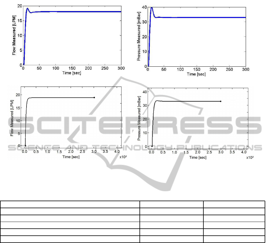
The flow and pressure curves on the Simulink en-
vironment can be observed in Figs. 5(a) and 5(b). On
the Ptolemy environment, the same curves are shown
in Figs. 5(c) and 5(d), respectively.
In both simulation environments, the value ex-
pected in stead state for the experimental platform
has been reached. However, in the transient regime
were observed a smaller overshoot in Ptolemy than in
Simulink. This result can make it difficult to predict
what is really expected in the transient regime, which
is a critical regime in control applications.
Besides, on the Ptolemy environment there were
difficulties during the execution of the PI controller
within the state refinements. Therefore, it was neces-
sary to build the basic structure of the controller using
gain and integrators blocks to operate in a more inter-
nal model.
Despite the fast execution of the simulation model
in Simulink, this computational tool did not able to
reproduce FSMs in the model. In this case, it would
require the addition of the Simulink function blocks
within Stateflow, which is other simulation environ-
ment specifics to work with logic and state machines.
Relative to the evaluation of the learning tools, the
engineering students analyzed the criteria adopted af-
ter to realize the modeling of the engineering system
in study in both software environments, as shown in
Table 1.
Figure 3: The simulation model (main model and subsystems) obtained in Simulink to control the didactic platform in study
(Subsystem A: Subsystem referred to Gp11; Subsystem B: Subsystem referred to Gp12; Subsystem C: Subsystem referred to
Gp21; Subsystem D: Subsystem referred to Gp22).
CSEDU2015-7thInternationalConferenceonComputerSupportedEducation
228
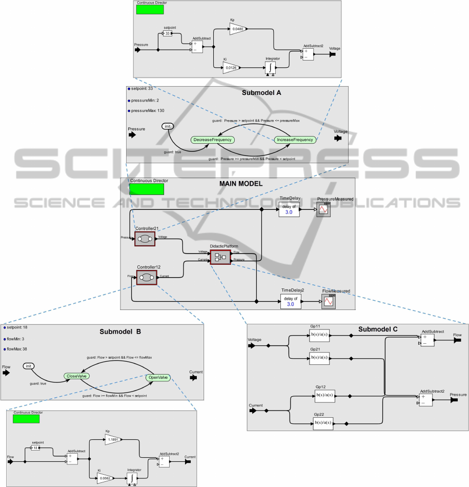
Figure 4: The simulation model (main model and submodels) obtained in Ptolemy to control the didactic platform in study
(Submodel A: Submodel referred to Controller21; Submodel B: Submodel referred to Controller12; Submodel C: Submodel
referred to DidacticPlatform).
SoftwareEnvironmentsasLearningToolsforModelingEngineeringSystems-ACaseStudyonDecentralizedMulti-loop
ControlSystem
229
(a) (b)
(c) (d)
Figure 5: (a) The flow curve and (b) the pressure curve obtained in Simulink; (c) The flow curve and (d) the pressure curve
obtained in Ptolemy.
Table 1: Criteria evaluated by engineering students about the learning tools used.
Criterion Simulink Environment Ptolemy Environment
The effort to build models Low High
The support material available High High
The level of knowledge about the tool High Low
The facilitate to analyze the engineering system behavior High Low
The spent time during the activity Low High
7 CONCLUSIONS
This work shown the implementation of simulation
models in different software environments for the
study of a decentralized multi-loop control system on
a fouling detection didactic platform. Besides, the
control system was considered as a CPS in both learn-
ing tools, in which enable engineering students simu-
late with more fidelity the system behavior.
On the Simulink environment, the simulation
model was based in a block diagram model using only
continuous dynamics. On the Ptolemy environment,
the simulation model was generated by means of hier-
archical actors models, with continuous and discrete
dynamics.
From the technical results, the simulation model
implemented in Ptolemy II was more complete, be-
cause this model was able to represent in greater de-
tail the hybrid behavior of the control system in study.
However, based in the learning results, the choice of
the best software environment was associated to the
engineering student experience in the tool, because
this criterion has facilitated in the construction and
the understanding of the model obtained.
Therefore, mathematical models implemented in
software environments have proven to be a powerful
tool for teaching simulation of engineering systems.
CSEDU2015-7thInternationalConferenceonComputerSupportedEducation
230

ACKNOWLEDGEMENTS
The authors would like to thank CNPq and PPgEE-
COPELE for financial support to the development of
this project.
REFERENCES
Derler, P., Naderlinger, A., Pree, W., Resmerita, S., and
Templ, J. (2008). Simulation of let models in simulink
and ptolemy. In Monterey Workshop. Budapest.
Despotovi-Zraki, M., Bara, D., Bogdanovi, Z., Jovani, B.,
and Radenkovi, B. (2014). Software environment for
learning continuous system simulation. Acta Polytech-
nica Hungarica, 11(2):187–202.
He, M.-J., Cai, W.-J., Ni, W., and Xie, L.-H. (2009). Rnga
based control system configuration for multivariable
processes. Journal of Process Control, 19:1036–1042.
IEEE, C. S. (1990). Ieee standard glossary of software en-
gineering termilogy. IEEE Standards Board.
Lee, E. A. (2014). Constructive models of discrete and con-
tinuous physical phenomena. IEEE Access, 2:797–
821.
Mosterman, P. J., Zander, J., Hamona, G., and Denckl, B.
(2012). A computational model of time for stiff hy-
brid systems applied to control synthesis. Control En-
gineering Practice, 20:2–13.
Ptolemaeus, C. (2014). System Design, Modeling, and Sim-
ulation using Ptolemy II. Creative Commons, Califor-
nia, USA, 1st edition.
SoftwareEnvironmentsasLearningToolsforModelingEngineeringSystems-ACaseStudyonDecentralizedMulti-loop
ControlSystem
231
