A Method for Managing Transportation Requests and Subdivision Costs
in Shared Mobility Systems
Gianmichele Siano, Mariano Gallo and Luigi Glielmo
Universit´a degli studi del Sannio, Benevento, Italy
Keywords:
Shared Mobility Systems, Ridesharing, Shapley Value, Optimization Vehicle Routing.
Abstract:
This paper presents an algorithm for managing the demand and supply in a shared transportation system. In
particular we present a method, independent from the Geographic Information System (GIS), which processes
drivers and passengers requests and ranks them in order to encourage matching and to propose the solution
profitable for all. The basic idea is to give priority to the requests of passengers with more common route and
avoid those with greater excess path. In the end, we propose a solution for the distribution of costs among the
participants of shared travel based on the application of the Shapley value.
1 INTRODUCTION
In recent years, the business models based on shared
economy and collaborative consumption are develop-
ing worldwide. Thanks to the massive use of the Inter-
net, Smartphone and associated technologies such as
GPS, GIS and Social Networks, which allow to com-
municate in real time and know immediately the geo-
graphical position.
Also in the transport sector systems are under de-
velopment with the objective of sharing private cars
among a groups of people who have a similar journey.
The main aim is to promote the sustainable mobility
and reduce transportation costs, traffic congestion and
pollution.
In a shared transport system, typically a driver
makes available to potential passengers the empty
seats of his/her vehicle. To use the service, the pas-
sengers help by paying adequate costs, generally pro-
portional to the shared journey. These systems are
generally called Carpool or Ridesharing.
In this paper we will refer to real-time Rideshar-
ing where the matching between the participants can
also take a few minutes before departure or during the
journey itself.
The objective of this work is to describe an op-
timization algorithm that can process requests from
participants in the system and classify them in order
to propose a solution beneficial for all.
Given a number of drivers offers and passengers
requests, the problem is how to combine these de-
mands efficiently and how to determine which of the
different options are the best for each individual sub-
ject.
Since a driver and one or more passengers share
different paths, another problem addressed in this pa-
per is to define an impartial method for the subdivi-
sion of transport costs.
The study of the problems described above has
been addressed in several previous studies, in partic-
ular in (Son et al., 2012) where an algorithm has been
proposed “based on labeling algorithms for solving
the multiobjective shortest path problem”, another so-
lution (Sghaier et al., 2010) uses an algorithm based
on “Distributed Dijkstra based on the multi-agent”
concept. In (Guo et al., 2012) a “Genetic Adaptive
algorithm” was used, while in (Calvo et al., 2004) a
system is presented using web GIS and SMS where
the problem of carpooling is solved with a heuristic
algorithm. Also in (Ferrari et al., 2003) a “Heuris-
tic algorithms based on savings functions” was pro-
posed. Finally (Santi et al., 2014) has been showed
and quantified “the benefits of vehicle pooling with
shareability networks”.
The paper is organized as follows. In the sec-
ond section we discuss the algorithm implemented in
all the critical steps, then we show the temporal se-
quence and the communications between the parteci-
pants, finally we propose a hypothesis of system ar-
chitecture and an example of algorithm usage. In the
third phase we discuss the problem of the cost dis-
tribution and propose a method based on the “Shap-
ley value”. Finally an example of application of this
method is showed.
152
Siano G., Gallo M. and Glielmo L..
A Method for Managing Transportation Requests and Subdivision Costs in Shared Mobility Systems.
DOI: 10.5220/0005459501520158
In Proceedings of the 1st International Conference on Vehicle Technology and Intelligent Transport Systems (VEHITS-2015), pages 152-158
ISBN: 978-989-758-109-0
Copyright
c
 2015 SCITEPRESS (Science and Technology Publications, Lda.)

2 MANAGING
TRANSPORTATION REQUESTS
2.1 Problem Description
In Figure 1 the typical representation of the problem is
shown, where in a certain geographical area, there is
a driver who intends to start from a position D
start
and
wants to reach the position D
end
, given a departure
time T
D
. The driver has available a certain transport
capacity C
max
equal to the maximum number of seats
available in the car.
In addition to the driver, in the figure there are 3
requests of passengers (P1, P2, P3), with the relative
position of origin and destination indicated by Pi
start
e Pi
end
and the respective departure times T
Pi
.
The basic idea of the method is to define a crite-
rion to prioritize the requests of passengers and quite
reasonably we propose to avoid those with greater ex-
cess path. For excess path we mean the extra path the
driver has to travel to pick up the passenger from her
starting position and to accompany him to her desti-
nation.
Given two generic data points P and Q, where
each point is characterized by geographical latitude
and longitude, e.g. P = (lat
P
;lng
P
), denote by
length(P, Q) the distance, along the path, between P
e Q obtained by querying a GIS, and by dist(P, Q) the
distance “as the crow flies” calculated according to
the formula:
dist(P, Q) = Rarccos[sin(lat
P
)sin(lat
Q
)+
+ cos(lat
P
)cos(lat
Q
)cos(lng
P
− lng
Q
)]
(1)
where R is the radius of the Earth. The value of dist
not depends from GIS, but from the geographical co-
ordinates transfered by drivers and passengers.
2.2 Proposed Solution
In Figure 2 we show the flowchart of the proposed
algorithm, hereinafter we will be describe in detail the
functionality of each block.
2.2.1 Input Block
Passing (D
start
, D
end
) to the GIS it is possible to get
the driver route DR and the total travel time T
D
.The
effects of traffic jam are not explicitly considered, but
depends by GIS utilized. DR is completely described
by the set of K points that compose it through a spatial
sampling:
Figure 1: Typical situation.
DR
P(k) per k = 1, . . . , K where
(
DR
P(1) = D
start
DR
P(K) = D
end
(2)
Given the definitions described in the previous
section inputs to our system will be:
• Driver: D
start
, D
end
, DR
P(k), T
D
,C
max
• Passengers: Pi
start
, Pi
end
, T
Pi
2.2.2 Eligible Passengers
This block will be used to select those passengers
whose requests are comparable in terms of both dis-
tance and timing.
In particular the i-th passenger, will be eligible in
terms of time (time-wise) if her date and time of de-
parture is subsequent to those of the driver. If we de-
note by T
D
the starting time of the driver and T
Pi
the
time of departure of the passenger, the constraint will
be expressed as:
T
Pi
≥ T
D
. (3)
The i-th passenger will be considered eligible in
terms of distance (distance-wise) if
length(D
start
, D
end
) ≥ α∗ dist(Pi
start
, Pi
end
) (4)
where α ≥ 1 is a tunable parameter and
dist(D
start
, Pi
start
)+dist(D
end
, Pi
end
) ≤ length(D
start
, D
end
)
(5)
Inequality (4) is used to eliminate those passen-
gers whose route is much longer than the driver’s (e.g.
α = 1.1), while inequality (5) is important because it
AMethodforManagingTransportationRequestsandSubdivisionCostsinSharedMobilitySystems
153

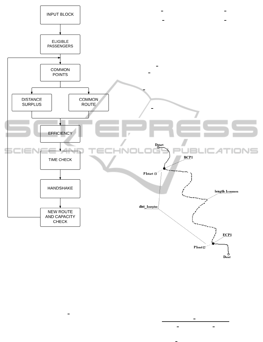
Figure 2: Flow chart.
helps to remove most passengers whose route direc-
tion is opposite to that of the driver’s (e.g. passenger
3 in figure 1 would be excluded).
Once the system identified the eligible passengers,
the ranking operations will start.
2.2.3 Common Points
Given all the data points associated to the geograph-
ical location of the driver DR
P(k), the first step of
the loop is to determine for each eligible passenger Pi
the points of the path DR with minimum distance (as
the crow flies), Pi
start
and Pi
end
. We denote this points
“Begin Common Point” (BCPi) and “End Common
Point” (ECPi), respectively. The associated equations
are
BCPi = DR
P(arg min
j
[dist(Pi
start
, DR P( j))])
ECPi = DR
P(arg min
j
[dist(Pi
end
, DR P( j))])
(6a)
(6b)
2.2.4 Distance Surplus and Common Route
Once we know the common points for the i-th
passenger, you can calculate the distance in ex-
cess, dist
i
surplus
, and the length of common route
length i
common
dist
i
surplus
= dist(P
start
, BCPi) + dist(P
end
, ECPi)
(7)
length
i
common
= length(BCPi, ECPi) (8)
In Figure 3, relatively to the passenger P1,the dis-
tance in excess has been drawn with a dotted line with
a dash-dot line.
Figure 3: Distance surplus and length common.
2.2.5 Efficiency
Distances are used to sort the various passengers ac-
cording to a value of efficiency:
Eff
i
=
length
i
common
length i
common
+ γdist i
surplus
(9)
This value Eff
i favors passengers who have long
common route and short surplus distance. The value
of γ depends on the preferences of the driver, who de-
cides what weight to attribute to route excess com-
pared to the common one.
VEHITS2015-InternationalConferenceonVehicleTechnologyandIntelligentTransportSystems
154

2.2.6 Time Check
Afterwards the algorithm checks whether the driver
arrives at the starting point of the passenger later than
the desired starting time of the passenger; this condi-
tion can be approximately checked as
T
Pi
≤ T
D
+T
DR

arg[BCPi]
K
+
dist(BCPi, Pi
start
)
length(D
start
, D
end
)

(10)
2.2.7 Handshake
In this block, the system notifies the driver with a
sorted list according to the metrics described above;
then, the system awaits the decisions of the driver and
passenger. The step of decision and agreement will
be described later (subsection 2.4).
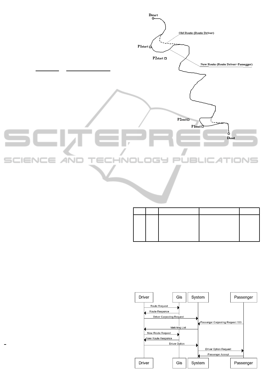
2.2.8 New Route and Capacity Check
If the actors reach an agreement, the passenger is
added to the shared travel and the capacity is decre-
mented by one.
A new request is made to the GIS for the exact
route calculation, all associated values and resulting
rescheduling times. This new request takes into ac-
count the passage through the begin and end points of
the chosen passenger.
In Figure 4 we show how the route is changed after
addition of the passenger P1.
This operation will be repeated recursively until
either the driver does not detect any potential passen-
ger or the numbers of places available si zero.
2.3 Example
In this example we show the operations of the algo-
rithm described above where γ = 4, in this case for
simplicity the time variable is not considered. For the
driver:
• D
start
= Napoli(40.8517763, 14.2681383)
• D
end
= Milano(45.4654323, 9.1859402)
• length(D
start
, D
end
) = 773, 74 km
• K = 12651
In (DRPK, 2014) you can find (lat,lng) data of
DR
P(k) of the route (Napoli,Milano). These data are
found using GIS (GoogleMaps, 2014).
Further, we constructed a list of hundred of pas-
sengers randomly generated. For every passenger the
towns of departure and arrival with the relative geo-
graphic locations are known:
Figure 4: Old Route and new Route.
• i,(lat
P
start
, lng
P
start
), (lat
P
end
, lng
P
end
)
This information is in (data.cvs, 2014)
The Table 1 below shows the first 4 passengers of
the sorted list.
Table 1: First four passengers.
N i BCP ECP Eff
P
1
10 44.473,11.270 45.349,9.310 0.960
P
2
32 40.854,14.318 43.779,11.161 0.801
P
3
81 40.869,14.321 45.168,9.598 0.792
P
4
88 41.996,12.671 44.524,11.151 0.756
2.4 Time Sequence
Figure 5 showns the time sequence of the algorithm
described above.
Figure 5: Time Sequence.
AMethodforManagingTransportationRequestsandSubdivisionCostsinSharedMobilitySystems
155

The driver initially, known geographic locations
of departure D
start
and destination D
end
, sends a re-
quest to the GIS (Route Request), which responds
by transmitting information about the different pos-
sible routes (Route Response). Each route con-
tains the travel path DR (Driver Route), the length
“length(D
start
, D
end
)”, the travel time T
D
and all points
DR
P(k).
The driver selects the most appropriate route and
informs the central system which performs the al-
gorithm. The system processes the driver request
(Driver Carpooling Request).
At a later time a generic passenger i with geo-
graphic location of departure Pi
start
and desired des-
tination Pi
end
sends its own request to the central sys-
tem (Passenger Carpooling Request).
The system evaluates the different requests of pas-
sengers and transmits to the driver the sorted list
(Matching List) based on the algorithm previouslyde-
scribed.
When a passenger has been chosen the driver
sends a new request to the GIS (New Route Request).
The GIS replies with a new route, that starts from the
starting point of the driver, passes through the points
of origin and destination of the passenger and ends
with the destination of the driver. (New Route Re-
sponse).
Comparing information between old and new path
it is possible to know with precision the true path ex-
cess, the true common path and the economic bene-
fits.
This option, with the correspondingeconomic val-
ues, is communicated to the System (Driver Option).
The System notifies the passengers (Driver Option
Request) who decides whether accepting the proposal
or not (Passenger Accept).
2.5 Architecture
Figure 6: Architecture.
Figure 6 shows a possible system architecture.
The devices (Driver/Passenger Device) that interact
with the system can be Smartphone, PC, PDA, Tablet
or other. Some of these systems may have an Internal
GIS others instead require an internet connection to
send requests to gis (External GIS).
Note that in this architecture the system that man-
ages the different request of the drivers and passen-
gers does not require direct communication with the
GIS.
3 COST SUBDIVISION
3.1 Problem Description
In shared trasportation system an important problem
is how to evaluate a fair division of the costs as func-
tion of the journeys in common among the various
participants.
Figure 7: Different shared paths.
Figure 7 is shows an example where a driver and
three passengers share different paths
For the solution of the problem we used a method
based on the “Shapley value” (Osborne and Rubin-
stein, 1994), which given a coalition and an associ-
ated payoff redistributes the payoffs in proportion to
the contribution that each player gives to the coali-
tion. An important property of the Shapley value is
that it considers the order of the player joining the
coalition in computing their respective contribution to
the “coalition”.
3.2 Shapley Value
In a shared transportation system the model of the
driver and passengers is comparable to a cooperative
game, with transferable utility and superadditivity.
Given N, the set of players (driver D and passen-
gers Pi) with |N| ≥ 2 and S, R two generic coalitions
S, R ⊆ N, define v the characteristic function, i.e. the
cost coalition S has to pay to make the shared journey.
Given a path length d
route
and a travel time t
route
we can calculate the cost associated approximately as:
c
route
= β
1
∗ d
route
+ β
2
∗ t
route
(11)
where β
1
is a coefficient that considers the type of
route and β
2
considers the time spent for moving (in
Italy, β
1
is variable from a minimum of 0.06 e/km
VEHITS2015-InternationalConferenceonVehicleTechnologyandIntelligentTransportSystems
156

for motorways to a maximum of 0.12 e/km for city
driving and β
2
is 15-20 e/h for working time and 7
e/h for holiday time).
Thus in our case the characteristic function has
the following properties, required to apply Shapley’s
method:





v(
/
0) = 0
v(S∪ R) < v(S) + v(R) if D ∈ S or D ∈ R
v(S∪ R) = v(S) + v(R) otherwise
(12)
The cost of coalition composed by only passengers is
a sum of the cost associated to the single passenger.
In other words coalitions including a driver and pas-
sengers have a total cost which is less than the sum
of subcosts; if, instead, neither coalition includes a
driver, the total cost is the sum of costs.
The Shapley value is used for distributing the to-
tal cost of the coalition among its members and aims
to subdivision in proportion to the marginal cost that
each player adds to the coalition.
First we need to calculate all the possible order-
ings of N elements and then we make an average of
all the marginal costs of the individual player on all
orderings previously calculated. The value of N is in-
cremented by one every time we add a new passenger
to the coalition.
This value is calculated using:
φ(i) =
1
|N|!
∑
π∈Π
N
[v(B(π, i) ∪ {i}) − v(B(π, i)] (13)
where:
• φ(i) Cost of the i-th participant to shared travel;
• Π
N
Set of all possible orderings of the elements
of N (permutations);
• B(π, i) is the set of players in N which precede the
player i in the ordering considered.
3.3 Example
Suppose there is a driver and two passengers, the total
cost is calculated using (11) where β
1
= 0.09 e/km
and β
2
= 0 e/h. For the computation of d
route
using
(GoogleMaps, 2014).
Table 2 summarizes the input data.
Table 2: Example 1: Input Data.
Users Begin End Cost e
D Napoli Milano 69.57
P
1
Caserta Bologna 49.68
P
2
Roma Firenze 25.02
Table 3: Example 1: Characteristic function.
User Cost e
D 69.57
P1 49.68
P2 25.02
D, P1 72.27
D, P2 72.63
P1, P2 74.70
D, P1, P2 75.33
Table 4: Example 1: Solution.
User Shared cost e Saving
D 35.1 49.55 %
P
1
26.19 47.28 %
P
2
14.04 43.88 %
Using the input data we can build the characteris-
tic function, respecting (12). The Table 3 shows the
associated cost for each coalition.
Table 4 reports the costs distributed according to
Shapley’s value using (13).
Another example of cost calculation using this
method and the data in (solution.cvs, 2014) is shown
in Table 5.
Table 5: Example 2: Solution.
User Initial cost Shared cost e Saving
D 69.57 9.19 86.8 %
P
1
45.0 24.85 44.77 %
P
2
17.28 9.13 47.19 %
P
3
38.16 21.13 41.9 %
P
4
36.36 21.13 41.9 %
4 CONCLUSIONS
In this article we studied the problem of shared trans-
port system, in particular we proposed an algorithm
that can process requests from players in the system
and rank them in order to propose the solutions bene-
ficial for all.
The algorithm implemented favors the demands of
passengers with longer route in common and avoid
those with greater excess path. The algorithm is in-
dependent of GIS, because the system works with the
GIS data requested by driver.
Finally a solution to the problem of cost-sharing
among participants in a shared transport system based
on the application of Shapley’s value was exposed.
For this method, a patent application was pre-
sented (Siano et al., 2014).
AMethodforManagingTransportationRequestsandSubdivisionCostsinSharedMobilitySystems
157

REFERENCES
Calvo, R., de Luigi, F., Haastrup, P., and Maniezzo, V.
(2004). A distributed geographic information system
for the daily carpooling problem. Computers and Op-
erations Research V.31, I.13, pp. 2263-2278.
data.cvs (2014). https://drive.google.com/file/d/0B
mFY
m1leYv9Q05SN0g4bzdmdjA/view?pli=1.
DRPK (2014). https://drive.google.com/file/d/0B
mFY
m1leYv9OHRzYU9qOFJLUnM/view?usp=sharing.
Ferrari, E., Manzini, R., Pareschi, A., Persona, A., and Re-
gattieri, A. (2003). The car pooling problem: Heuris-
tic algorithms based on savings functions. Journal of
Advanced Transportation V.37, I.3, pp. 243-272.
GoogleMaps (2014). https://www.google.it/maps/dir/
Napoli/Milano.
Guo, Y., Goncalves, G., and Hsu, T. (2012). A multi-agent
based self-adaptive genetic algorithm for the long-
term carpooling problem. Journal of Mathematical
Modelling and Algorithms in Operations Research,
V.12, I.1, pp. 45-66.
Osborne, M. and Rubinstein, A. (1994). A course in Game
Theory. The MIT Press, Cambridge, Massachusetts.
Santi, P., Resta, G., Szell, M., Sobolevsky, S., Strogatz, S.,
and Ratti, C. (2014). Quantifying the benefits of vehi-
cle pooling with shareability networks. PNAS V.111,
pp. 13290-13294.
Sghaier, F., Zgaya, S., Hammadi, T., and Tahon, F. (2010).
A distributed dijkstra’s algorithm for the implemen-
tation of a real time carpooling service with an opti-
mized aspect on siblings. IEEE Annual Conference
on Intelligent Transportation Systems.
Siano, G., Gallo, M., and Glielmo, L. (2014). Algo-
ritmo per la gestione di un sistema di carpooling. N.
BN2014A000012, CCIAA di Benevento Cod. 62.
solution.cvs (2014). https://drive.google.com/file/d/0B
mF
Ym1leYv9NkxnWkNUeGdfa2M/view?usp=sharing.
Son, T., An, L., Tao, P., and Khadraoui, D. (2012). A
distributed algorithm solving multiobjective dynamic
carpooling problem. International Conference on
Computer Information Science.
VEHITS2015-InternationalConferenceonVehicleTechnologyandIntelligentTransportSystems
158