
Traffic Flow Prediction from Loop Counter Sensor Data using
Machine Learning Methods
Blaž Kažič, Dunja Mladenić and Aljaž Košmerlj
Artificial Intelligence Laboratory, Jožef Stefan Institute, Jamova cesta 39, 1000 Ljubljana, Slovenia
Keywords: Time Series, Traffic Flow Prediction, Feature Engineering, Ridge Regression, SVR, Random Forests.
Abstract: Due to increasing demand and growing cities, traffic prediction has been a topic of interest for many
researchers for the past few decades. The availability of large amounts of traffic-related data and the
emerging field of machine learning algorithms has led to a significant leap towards data-driven methods. In
this paper, loop counter data are used to develop models that can predict traffic flow for several different
prediction intervals into the future. In depth exploratory data analysis and statistical testing is performed to
obtain good quality informative features. Several feature sets were compared by using different machine
learning methods: Ridge Regression, SVR and Random Forests. The results show that in order to obtain
good prediction results thorough feature extraction is just as or even more important than learning method
selection. Good features enables us to use less complex methods, which run faster, are more reliable and
easier to maintain. In conclusion, we address ideas regarding how predictions could be improved even
further.
1 INTRODUCTION
Traffic congestion can have substantial effects on
quality of life, especially in bigger cities. It is
estimated that traffic congestion in United States
causes two billion gallons of fuel to be wasted every
year; 135 million US drivers spend two billion hours
stuck in traffic every year. Altogether, 100 billion
USD are spent because of fuel in the US alone. For
an average American driver, this costs 800 USD per
year (Liu et al., 2006). In addition to economic
aspect (wasting money and time), there is also an
ecological one. Pollution could be reduced
significantly by reducing travel time and thus
emissions.
The above mentioned facts are the main reasons
that governments are investing in Intelligent
Transportation Systems (ITS) technologies that
would lead to more efficient use of transportation
networks. Traffic prediction models have become a
main component of most ITS. Accurate real time
information and traffic flow prediction are crucial
components of such systems. ITS vary in
technologies applied in; from advanced travel
information systems, variable message signs, traffic
signal control systems, to special user-friendly
applications, such as travel advisors. The aim of all
of these technologies is the same, to ease traffic
flow, reduce traffic congestion and decrease travel
time by advising drivers about their routes, time of
departure, or even type of transportation
(Stathopoulos and Karlaftis, 2003).
The availability of large amounts of traffic-
related data, collected from a variety of sources and
emerging field of sophisticated machine learning
algorithms, has led to significant leap from
analytical modelling to data driven modelling
approaches (Zhang et al. 2011). The main concept of
this paper is to investigate different machine
learning algorithms and engineer features that would
enable us predicting traffic state several prediction
intervals into the future.
2 RELATED WORK
In general, traffic prediction studies can be
categorized into three major categories: naïve
methods, parametric methods and non-parametric
methods (Van Lint and Van Hinsbergen, 2012).
Naïve methods are usually simple non-model
baseline predictors, which can sometimes return
good results. Parametric models are based on traffic
flow theory and are researched separately and in
119
Kažic B., Mladeni
´
c D. and Košmerlj A..
Traffic Flow Prediction from Loop Counter Sensor Data using Machine Learning Methods.
DOI: 10.5220/0005495001190127
In Proceedings of the 1st International Conference on Vehicle Technology and Intelligent Transport Systems (VEHITS-2015), pages 119-127
ISBN: 978-989-758-109-0
Copyright
c
2015 SCITEPRESS (Science and Technology Publications, Lda.)

parallel to non-parametric, more data-driven
machine learning methods.
A strong movement towards non-parametric
methods can be observed in the recent years,
probably because of increased data availability, the
progress of computational power and the
development of more sophisticated algorithms
(Vlahogianni et al., 2014). Non-parametric does not
mean models are without parameters; but refers to
model’s parameters, which are flexible and not fixed
in advance. The model’s structure as well as model
parameters are derived from data. One significant
advantage of this approach is that less domain
knowledge is required in comparison to parametric
methods, but also more data is required to determine
a model. This also implies that successful
implementation of data-driven models is highly
correlated to the quality of available data.
Non-parametric methods can be further
subdivided into two subgroups: classical statistical
regression approaches and data-driven machine
learning approaches (Karlaftis and Vlahogianni,
2011). From the group of statistical methods, the
local linear regression algorithm yields surprisingly
good results, especially on highway data (Rice and
van Zwet, 2004). In contrast, traffic in urban areas
can be much more dynamic and non-linear, mainly
because of the presence of many intersections and
traffic signs. In such environments, data-driven
machine-learning approaches, such as neural
networks (Van Hinsenberg et al., 2007) and SVR
(Vanajakshi and Rilett, 2007), can be more
appropriate, due to their ability to model highly
nonlinear relationships and dynamic processes. In
this research, we test methods from both groups:
statistical regression approaches and more complex
nonlinear algorithm.
3 DATA
The data used in this research is collected by a single
traffic counter sensor, installed inside the bypass of
Ljubljana, the capital city of Slovenia.
Measurements are available via a web API service
(http://opendata.si/promet/), as a real-time data
stream, refreshed every 5 minutes. Our collected
database consists of 6-month record set of sensor
data (from January 2014, to July 2014), amounting
to 46,447 records.
Every record consists of a timestamp, descriptive
information about the sensor (location, region,
direction, etc.), and the five different measurements
used in this research:
Flow: the number of vehicles passing certain
reference point, per hour.
Gap: average time gap (in seconds) between
vehicles, per hour.
Occupancy: occupancy of the road in the
value of 1/10th of one percent, e.g. value 57
from the data converts to 5.7 %.
Speed: average speed (km/h) of vehicles, per
hour. The speed of every vehicle is almost
impossible to track and is, therefore, estimated
from other parameters.
Traffic status: Numeric status of the traffic. 1
being “normal traffic”, and 5 being “heavy
traffic with congestion”.
Figure 1: Traffic loop sensor data for randomly selected week.
VEHITS2015-InternationalConferenceonVehicleTechnologyandIntelligentTransportSystems
120

3.1 Data Preprocessing
Upon the first audit of the collected measurements,
we determined that many records were duplicated
during the 5-minute intervals. Since the timestamp
was duplicated as well, we can assume these are
actually missing values, probably due to service
downtime.
With further sanity checking of data, it became clear
that several entries also contain clearly wrong or
invalid values. For example, we know that the
“TrafficStatus” parameter can have only values
between 1 and 5, but in our data, some values was 0.
After checking this records’ data, we have
determined that other measurements for this record
had been corrupted as well; therefore, all such
records were marked as invalid samples.
Missing data and records flagged as invalid data,
were handled with partial listwise deletion approach.
There are two reasons for this choice. First, since the
gaps in our missing data can be very long (from a
couple of hours to a couple of days), it is not trivial
to replace missing values, and we could induce too
much uncertainty by replacing missing records.
Second, after cleaning data with partial deletion
method, we have reduced the number of records in
the data set by 37%, but we are still left with a
reasonable large amount of data (29,215 samples) to
train and test our prediction models, on a much
cleaner and more representative data set.
3.2 Exploratory Data Analysis
By visually exploring the data of one randomly
selected week from our dataset (Figure 1), we can
distinguish daily patterns over the week. The
difference between traffic by day and traffic by night
is clearly seen. Another interesting observation is
that working days during the week have highly
similar pattern, while patterns for the weekend are
different. A distinguished peak in the morning
(morning rush hour), followed by another peak
(afternoon rush hour), can also be observed.
Another interesting finding that can be observed
from the graph below is the anomaly seen on
Wednesday during the afternoon rush hour. We can
observe a drop in the flow and speed parameters,
which means that the speed and traffic flow were
unusually low for that time at the day. Furthermore,
we can see that occupancy was very high at that time
and that the traffic status changed from status 4 to 5.
This is most probably due to traffic congestion
(traffic jam or accident). This is also the most
informative type of information to predict.
3.2.1 Traffic Flow during the Week
In the previous chapter, it was determined that traffic
during the weekend is significantly different than on
weekdays, which is intuitively understood to be true.
This implies that it would be useful to include this
information (whether it is weekend or weekday) in
the form of a new feature, when training our model.
What about traffic during the days in the week?
Would it also be useful to have the day of the week
as a feature?
In order to answer this question, we performed a
statistical T-test, with the assumption (null
hypothesis) that traffic flow during weekdays is the
same. Since the traffic flow parameter is non-
normally distributed, we performed Man-Whitney
U-test in order to test our null hypothesis. The p-
value, which determines statistical significance of a
hypothesis, was computed between all combinations
of days in the week. A small p-value (smaller than
the critical value, usually 0.05) means that we can
reject the null hypothesis; otherwise we cannot reject
it.
The results are presented in the form of a heat
map in Figure 2. We can see that the only
combinations for which we cannot reject our null
hypothesis (p-value > 0.05) are the days from
Tuesday to Thursday. However, we can reject our
null hypothesis for all other days, meaning that
traffic is significantly different for these days.
According to these results, it would make sense to
also include the day of the week as a feature in to
our model.
Figure 2: P-values from Man-Whitney test.
TrafficFlowPredictionfromLoopCounterSensorDatausingMachineLearningMethods
121
3.2.2 Average Traffic Flow
Another assumption, obtained from the data
analysis, is that the traffic state on a certain day and
time is similar to traffic one week ago at the same
time. From the historical data, we have calculated
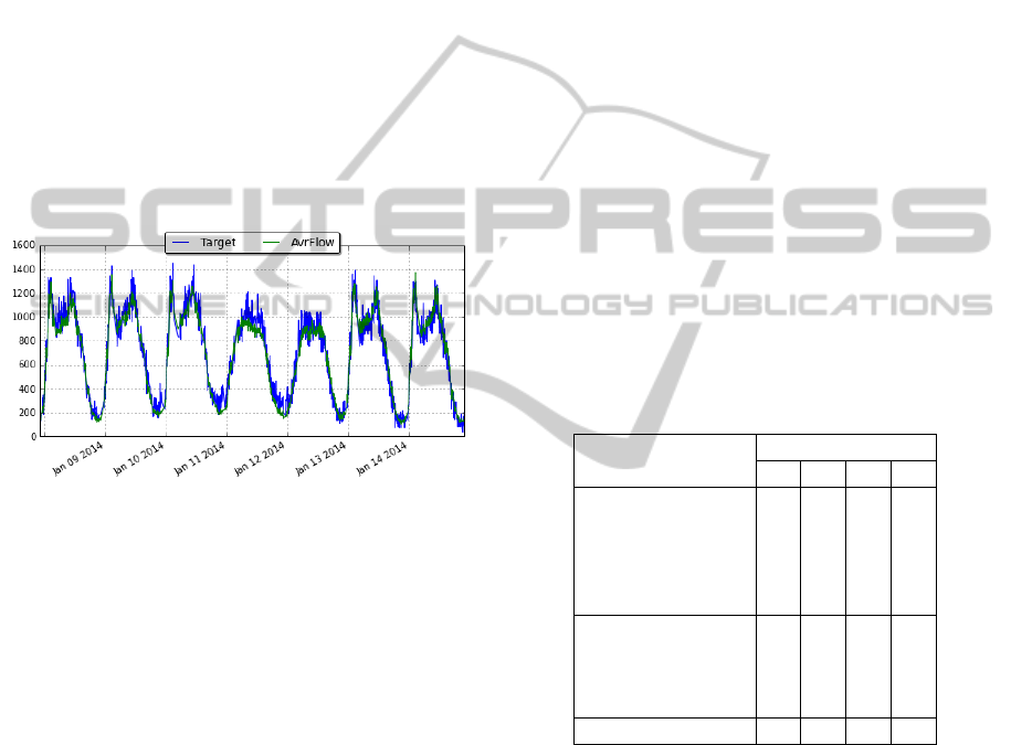
the averaged traffic status for our target variable (i.e.
flow) according to day and time over one week. In
the Figure 3, we can see the result and a comparison
between these data and one randomly selected
weekly data. It can clearly be seen that average
traffic is already a very good fit. In fact, this simple
naïve predictor is still widely used in various
practical applications, such as routing or travel time
estimation (Van Lint and Van Hinsbergen, 2012).
We will use this information as a feature when
training models and as a baseline predictor when
comparing different methods.
Figure 3: Traffic flow average for one week.
3.3 Feature Engineering
It is a well-known fact that feature engineering is a
key to success in applied machine learning. Feature
engineering is the process of transforming raw data,
into features that better represent the underlying
problem to the predictive models. Better the
features, better the results. The best way to extract
good representative features, is by exploring and
understanding, which is what we did in previous
section.
We have already discovered that there exists a
relationship between datetime and other attributes.
Since it can be difficult for a model to take
advantage of datetime native form (2014-01-01
01:00:00), we want to decompose a datetime into
consistent parts, that may be more informative for
the model. We introduce four new features:
HourOfDay [0 - 23]
DayOfWeek [0 - 6]
Month [0 -12]
Weekday/Weekend [0 - 1]
From previous empirical experiences, it can also
be beneficial for some models, to convert these
ordinal variables into dummy/indicator (categorical)
variables (i.e. “DayOfWeek” feature 3 is
transformed to 0001000).
Another important information, derived from
outcomes of previous chapter, is weekly traffic is
very similar. Therefore, traffic average (according to
time and day of week) can represent normal traffic
surprisingly well. This information can be used as
feature, that informs what is the traffic status on
average, on specific time in the future. For this
purpose we create extra feature:
AvrFlow
Although good feature engineering is very
important in order to achieve high-quality prediction
results, the actual success is a combination between
the model that we choose, the data, and the extracted
features that we use. In order to obtain the best
combination, 4 different datasets were created
(which contains which features can be seen in Table
1)
Table 1: Features and datasets used in further analysis
(white circles indicates dummy features): (1)
only_measurements, (2) with_datetime, (3)
dummy_datetime, (4) with_avr_dummy.
Features Data set
1 2 3 4
Flow ● ● ● ●
Gap ● ● ● ●
Occupancy ● ● ● ●
Speed ● ● ● ●
TrafficStatus ● ● ● ●
HourOfDay ● ○ ○
DayOfWeek ● ○ ○
Month ● ○ ○
Weekday ● ○ ○
AvrFlow ●
4 METHODS OF PREDICTION
In this research, we have tested three different data
driven methods, from a well-known machine
learning library scikit-learn (version 0.15)
(Pedregosa et al., 2011):
Ridge Regression: Computationally non-
demanding and fast method; can perform
surprisingly well, with proper feature
engineering.
SVR: Regression Support Vector Machine is
sophisticated non-linear machine-learning.
VEHITS2015-InternationalConferenceonVehicleTechnologyandIntelligentTransportSystems
122
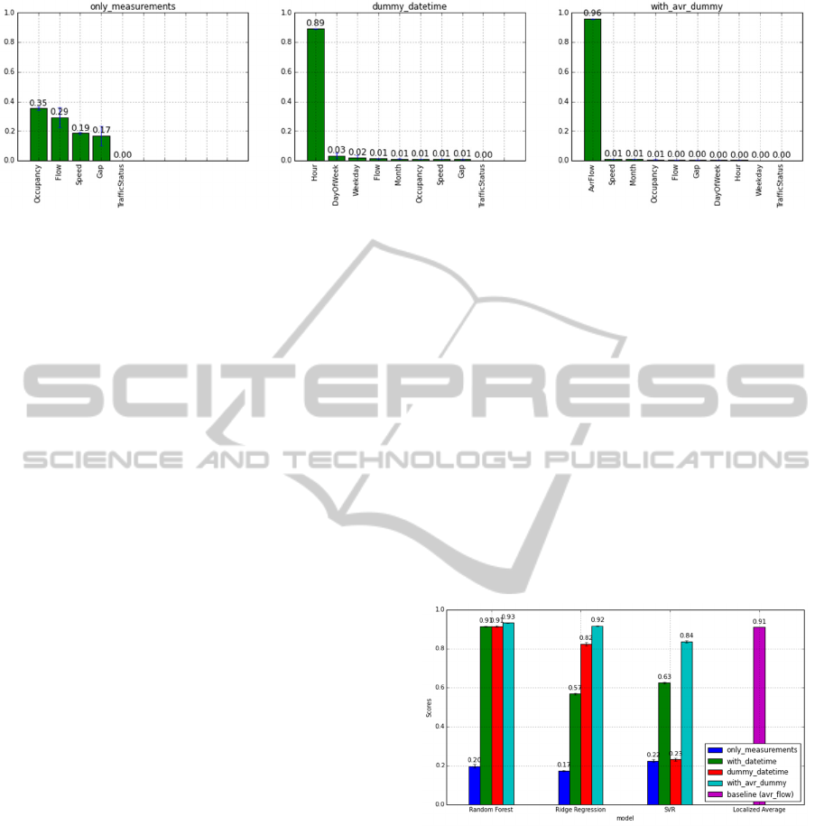
Figure 4: Feature importances for different data sets. We can observe how additional features change importances.
method, but can be computationally intense
and slow.
Random Forests: An ensemble method that
operates by constructing multitude of
decision trees. Usually needs some
parameter tuning to avoid over-fitting to
their training data.
In order to train models for comparison purposes,
we also need a target value, for which we want to
predict values. Since traffic flow is the most
informative attribute, in this research we used traffic
flow as a target attribute. We also need to specify the
prediction interval. For most part of this research, 5
hour interval was used. Target values were obtained,
by copying target attribute time series data, and
lagging it according to selected prediction interval
(in this case, 5 hours into the future). However, if
there is a need to predict any other attribute from the
database, or change the prediction interval, this is a
trivial task. At the end of this paper (results section),
performance with other prediction intervals have
been tested as well.
4.1 Method Comparisons
The performance of the above-described methods
with default parameter values was measured over a
range of different testing datasets (presented in
Feature Engineering chapter) by using measure of
fitness – coefficient of determination, denoted as R
2
.
This is a standard measure of accuracy for
regression problems. Values can range between -1
and 1, where score of value 1 implies a perfect fit
(Draper and Smith, 1998). When performing
comparison tests, cross validation method was used
(shuffled split, with 3 iterations, and testing size of
20 % of given data set). All tests also include a
baseline predictor used for comparison (average
traffic flow of one week, presented in Average
Traffic Flow chapter).
Comparing models over different datasets shows
how feature enrichment consistently improves
prediction scores with all methods (Figure 5). The
first major improvement in prediction performance
can be observed when using dataset with additional
features derived from datetime information (dataset
called with_datetime). Comparing to results where
only traffic measures are used (only_measurements),
R
2
score is approximately tripled for all methods.
This shows the significance of date time
information, which is intuitive, and it would be
absurd not to use it when dealing with time series
data. The importance of datetime-related features
can also be observed by performing a feature
importance test Figure 4, in which “HourOfDay”
feature is rated as the most important, followed by
“DayOfWeek” and “Weekend” features, also
extracted from datetime information.
Figure 5: Methods and feature sets comparisons.
Another interesting improvement can be observed
with the Ridge Regression method, when using
dummy datetime features (dummy_datetime).
According to previous experiences, this
improvement was expected, but it is interesting to
observe how the performance of the SVR model has
drastically decreased in comparison to the SVR
model that uses dataset in which datetime features
were not categorized (with_datetime). Losing the
order information of datetime variable values by
splitting them into separate independent variables
effectively nullifies their usefulness to SVR, as the
TrafficFlowPredictionfromLoopCounterSensorDatausingMachineLearningMethods
123

score drops back down to the same value as without
datetime information. Even when “avrFlow” is
available, the dummy features decrease the
performance in comparison to the baseline.
However, it is interesting that none of the above
mentioned results have over scored the baseline
predictor. In short, the reason for such good result of
the baseline method is the choice of a fairly long
prediction horizon, i.e. 5h into the future. This is
explained in greater detail later in the Results
section.
But the most important result is that by using
dataset where localized average flow as a feature
(feature set with_avr_dummy), Random Forests and
the Ridge Regression method have been able to
outperform the baseline method. The dominant
importance of the new feature “AvrFlow” can be as
well observed in Figure 4. From this figure we can
observe how feature importance has changed with
different datasets and it is clear that the “AvrFlow”
feature is by far the most important feature, when
predicting 5 hours into the future.
4.2 Learning Curves
By visualizing learning curves, we can have a better
look at developed models and diagnose whether our
model is performing well, or if it can be improved.
Figure 6 shows how SVR models need many more
examples to attain a good prediction score, while the
Ridge Regression and Random Forests methods
outperform it event when much less data is
available. According to the slope of the curve, we
can also assume that for these two methods, it does
not seems that the scores would improve with more
samples.
The fact that training and cross validation scores
are almost the same, can indicate that the model
suffers from high bias (is under-fitted). This
situation can be observed for Ridge Regression
performance with the “only_measurements” dataset
in Figure 6. Usually, this happens when we have an
abundance of data but too few features. One
standard way to improve the performance of such
model is by adding more features. Indeed, we can
observe that Ridge Regression prediction score has
increased significantly by adding additional features.
By looking at the Random Forests learning
curves, we can observe the gap between the training
and cross validation scores, which might indicate
that we are dealing with high variance (over-fitting).
In such cases, we might improve our model by
obtaining more training examples, by trying smaller
sets of features, or by decreasing complexity. Since
we do not have more training examples, we will
attempt to improve our model by taking into account
two other suggestions, by tuning the model
parameters.
Parameter optimisation was done by performing
a grid search over several different options for
different parameters: number of trees (n_estimators),
number of features (max_features), and minimum
Figure 6: Learning curves for several methods and different feature sets.
VEHITS2015-InternationalConferenceonVehicleTechnologyandIntelligentTransportSystems
124
number of samples in newly created leaves
(min_samples_leaf). The best parameter set was
found with 100 trees and with a minimum of 10
samples in leaves. With this optimisation, we have
significantly reduced the size of the decision trees
(from 26,013 to 2,207 nodes) and decreased
complexity, which makes this model simpler and
faster. This optimisation also resulted in a slightly
better prediction score (Occam’s razor).
Additionally, a well-known Ada Boost method
was also tested in order to determine if we could
significantly improve our score of the Random
Forests model. Indeed, the score was improved even
further from 0.93 to 0.94. Since this add-on also
significantly slowed down the performance, we
decided not to use it, but this result indicates we
could possibly improve our score even further.
5 RESULTS
The last 20% of the original data set was reserved
for evaluation purposes (15 May–30 Jun). What we
can clearly see from the results (Table 2) is the
general trend of how an additional feature set
consistently improves prediction performance over
all tested methods.
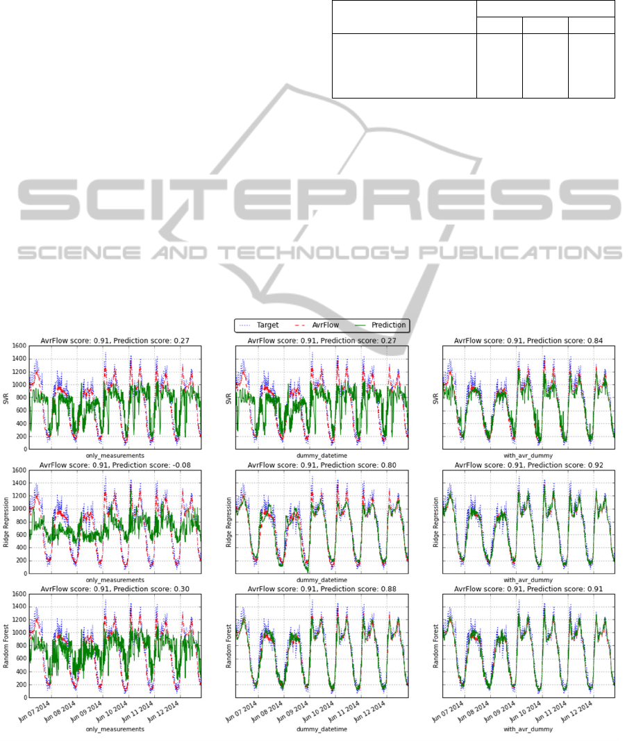
Table 2: R
2
score results for different models and datasets:
(1) only_measurements, (2) dummy_datetime, (3)
with_avr_dummy.
Method Data set
1 2 3
Historical Average 0.91 0.91 0.91
Ridge Regression -0.08 0.80
0.92
Random Forests 0.30 0.88 0.91
SVR 0.27 0.27 0.84
The results show that all models performed best
by using the “with_avr” feature set. By using this
testing dataset, Ridge Regression was the best
method (0.92), followed by Random Forest (0.91)
and baseline-average flow (0.91). Unlike in previous
cross validated test, when Random Forest was the
best prediction model, now Ridge Regression
performed better. This might infers that Random
Forest is indeed slightly over fitted. However, it is
again interesting to observe how well the baseline
method performed again in comparison to other
machine learning methods.
Figure 7: Visualizing predictions from different models, with different feature sets.
TrafficFlowPredictionfromLoopCounterSensorDatausingMachineLearningMethods
125

Figure 8: Error (MAE) comparison for different prediction horizons.
With additional analysis, we have encountered that
this is due to the relatively long predictive horizon
that we have chosen (5 hours into the future). Figure
8 show the prediction error (Mean Absolute Error -
MAE) results for three different models: two naïve
predictors and a linear regression model for several
prediction horizons (from 5 minutes to 12 hour into
the future). The first naïve predictor is the current
status predictor, which takes only current
measurements into account and assumes that traffic
will remain constant. The second is the localized
average traffic status, which was used as a baseline
in previous tests. The third model is Ridge
Regression, since it has been found to be the best
predictor in comparison to other methods in this
section.
From Figure 8 we can observe how current status
measurements works better than average status for
short-term predictions (prediction horizon less than
1h), while the average status works better for long-
term predictions, which is intuitively true, since the
current status has less influence on the long term.
The results also illustrate how the prediction error
increases with larger prediction horizons. This is
obvious as well, since larger forecast intervals
correspond to larger uncertainty.
However, the most significant point from this
figure is that linear regression outperforms both
naïve methods for all prediction horizons. This is
because this method indirectly includes both models
outputs (current status and average status) as
Figure 9: Traffic data with prediction errors.
inputs, and learns how to weight them according to
specific prediction horizons. Therefore, it makes
more accurate predictions.
By analysing predictions with the largest error
(Figure 9), we can conclude that most of them are
caused by anomalous traffic patterns, such as
holidays, or very low or high traffic (probably due to
traffic accidents or possibly bad weather). Since
average traffic is considered to be the most
important feature in our model (due to long
prediction interval - 5h), it is to be expected that we
experience the largest errors with anomalies. By
using additional data sources that could describe
such anomalous traffic, we could probably increase
our prediction accuracy. Examples of such
additional data sources would be information about
holidays, weather prediction reports, traffic status
reports, etc.
6 CONCLUSIONS
In this research, we have compared the performance
of three machine learning methods (Ridge
Regression, SVR, and Random Forests) used for
predicting traffic flow. Feature engineering was also
described and recognized as a key component for
good results.
The results show that simple naïve methods, such
as historical average, are surprisingly effective when
making long-term predictions (more than one hour
into the future), while using current traffic
measurements as naïve method for prediction works
well when making more short term predictions (less
than 1h). This is to be expected, since current traffic
situation effect more on traffic in the nearby future,
then on traffic in a few hours or days. What is more
important is, that results shows, that by using
machine learning methods which includes both;
historical averages and current values, predictions
are better than both previously mentioned naïve
predictors, for all prediction horizons (short term
and long term).
VEHITS2015-InternationalConferenceonVehicleTechnologyandIntelligentTransportSystems
126

Also noteworthy is the fact that by constructing
high quality features, simple methods, such as linear
regression can work as well or even better than other
more sophisticated algorithms (such as Random
Forests, SVR, etc.). By using less complex models,
optimal model parameters are found more readily,
the models run a lot faster, and they are easier to
understand and maintain.
We also state that the main disadvantage of
models presented in this research, is its inability to
predict unusual traffic events. Even though common
traffic status is informative for a commuter in a new
environment, unusual traffic is the most informative
information for local commuter who is aware of
usual traffic. The main reason for this disadvantage
is that current models uses only historical traffic
data. Since, some of unusually traffic events are
caused by other related events (such as nearby traffic
accidents, bad weather, holidays, etc.), we believe
that by including additional data sources in the
model, prediction of such events could be
significantly improved.
Therefore, our future plan is to collect several
quality traffic related data sources (such as weather
forecasts, traffic alerts, special days statuses, bigger
social events, etc.) and fuse them with loop counters
data in order to generate better traffic prediction
models. We intend to test different data fusion
approaches, such as: early (or full) integration;
which transforms data sources into a single feature-
based table, late (or decision) integration; where
each data source give rise to a separate model and
predictions are later fused, and intermediate (or
partial) integration, where data are fused through
inference of a single joint model with a recent matrix
factorization based algorithms, providing very good
results in the field of bioinformatics (Žitnik and
Zupan, 2013).
ACKNOWLEDGEMENTS
This work was supported by Slovenian Research
Agency and the ICT Programme of the EC under
MobiS (FP7-318452).
REFERENCES
Draper, N.R. and Smith, H., 1998. Applied regression
analysis, New York: Wiley, 3
th
edition.
Van Hinsenberg, C.P.I., Lint, J.W.C. Van and Sanders,
F.M., 2007. Short Term Traffic Prediction Models.
Proc., 14th World Congress on Intelligent Transport
Systems: ITS for a Better Life.
Karlaftis, M.G. and Vlahogianni, E.I., 2011. Statistical
methods versus neural networks in transportation
research: Differences, similarities and some insights.
Transportation Research Part C: Emerging
Technologies, 19(3), pp.387–399.
Van Lint, J.W.C. and Van Hinsbergen, C.P.I.., 2012.
Short-Term Traffic and Travel Time Prediction
Models, in Artificial Intelligence Applications to
Critical Transportation Issues. Transportation
Research Circular, E-C168 (November).
Liu, Y. et al., 2006. A scalable distributed stream mining
system for highway traffic data. Knowledge Discovery
in …, pp.309–321.
Pedregosa, F. et al., 2011. Scikit-learn: Machine Learning
in Python. Journal of Machine Learning Research, 12,
pp.2825–2830.
Rice, J. and van Zwet, E., 2004. A simple and effective
method for predicting travel times on freeways.
Intelligent Transportation Systems, IEEE
Transactions, pp.200–207.
Stathopoulos, A. and Karlaftis, M.G., 2003. A multivariate
state space approach for urban traffic flow modeling
and prediction. Transportation Research Part C:
Emerging Technologies, 11(2), pp.121–135.
Vanajakshi, L. and Rilett, L.R., 2007. Support Vector
Machine Technique for the Short Term Prediction of
Travel Time. 2007 IEEE Intelligent Vehicles
Symposium, pp.600–605.
Vlahogianni, E.I., Karlaftis, M.G. and Golias, J.C., 2014.
Short-term traffic forecasting: Where we are and
where we’re going. Transportation Research Part C:
Emerging Technologies.
Zhang, J. et al., 2011. Data-Driven Intelligent
Transportation Systems: A Survey. IEEE Transactions
on Intelligent Transportation Systems, 12(4), pp.1624–
1639.
Žitnik, M. and Zupan, B., 2013. Data Fusion by Matrix
Factorization. IEEE Transactions on Pattern Analysis
and Machine Intelligence, pp.13.
TrafficFlowPredictionfromLoopCounterSensorDatausingMachineLearningMethods
127
