Spatial Temporal Relational Graphs on Connected Landscapes

Alan Kwok Lun Cheung

, David O’Sullivan

and Gary Brierley

School of Environment, University of Auckland, Auckland, New Zealand

Department of Geography, University of California, Berkeley, Berkeley, CA 94720-4740, U.S.A.

1 RESEARCH PROBLEM

The structure of computational spatial analysis has

mostly built on data lattices inherited from

cartography, where visualization of information takes

priority over analysis. In these framings, spatial

relationships cannot easily be encoded into traditional

data lattices. This hinders spatial analysis that

emphasizes how interactions among spatial entities

reflect mutual inter-relationships at a very basic level.

With this limitation, landscape compositions and

configurations can be appreciated further if a

topologically and temporally enabled data structure is

available. The aim of this research is to develop a data

structure and its associated analytical methods to

assess the connections and interactions of landscape

elements through time and space. This additional

layer of information will help us understand the

dynamics of processes happening within and between

components of landscapes.

2 OUTLINE OF OBJECTIVES

This research has the following objectives:

1) Establishing a topologically enabled data

structure using graph theory. The aim for this

portion of research is to develop a “piggy-back”

topological data structure which can be produced

from existing vector and raster dataset, thus

maximize the compatibility of the methods

developed in this research.

2) Examine landscape patterns and their dynamics in

the form of subgraphs from the data structure. The

graph data structure will be interrogated using

methods ranging from pair-wise change

monitoring (Graph Edit Distance) to more

complicated subgraph structure monitoring

(cliques, communities). The associated extraction

methods have to be adapted from currently

available mathematical graph tools.

3) Evaluate the prominence of subgraph patterns on

the landscape and explain them in the context of

geography and landscape ecology. Extraction of

subgraphs and numerical assessment of patterns

on their own might not be sufficient in explaining

patterns on the landscape. Here domain expert

knowledge will be utilized to link up concepts

from geography and landscape ecology with that

of our empirical results.

3 STATE OF THE ART

Despite the popularity and variety of spatial statistics,

its ability to appraise landscape connectivity theories

through spatial patterns has been limited. Instead they

are viewed and used as means to an end. Typical

spatial pattern analysis has been concerned primarily

with statistical distribution of individual types of

entities. In such operations, the mechanism for

describing relationships between types of entities

relies on comparison of clusters or accumulative

statistics. Patterns discovered using these procedures

provide significant insight into the composition of the

landscape, but far less about its configuration.

Processes that cause interactions and changes

between entities are not deciphered. As such,

extraction of “patterns” in this way remains relatively

superficial as description of distributions takes

priority over the possibility of identifying relational

processes. Thus accumulative statistics may not be

the most suitable framework for realizing the

conceptual idea of a connected landscape.

The concept of connected landscape comes from

landscape ecology. The term Landscape Ecology was

coined by Troll (1939) in an effort to frame enquiry

into interactions among elements and associated

processes that explain ecological patterns in

landscapes. At the early stages of its inception,

analyses were restricted to thought experiments on

conceptual models and small scale case studies due to

difficulties in the acquisition and processing of data.

With advances in computing power, renewed interest

has been evident, increasingly targeting the

implementation of concepts in a systematic manner.

The realization of concepts are restricted by the

availability of tools. Current GIS and remote sensing

represent landscape with two main types of data

Cheung A., O’Sullivan D. and Brierley G..

Spatial Temporal Relational Graphs on Connected Landscapes.

 2015 SCITEPRESS (Science and Technology Publications, Lda.)

structures: a field view in raster data, and a feature

view in vector data. Both structures developed when

static visualization of spatial information took

priority. Although spatial relationships in forms of

proximity and topology are embedded in these

structures, this information is often not utilized. More

process-oriented approaches necessitate the inclusion

of spatial relationships to operate effectively

(Takeyama and Couclelis, 1997).

Despite limited attention in the earlier years of

GIS, graph theory has shown promising results for

representing structural properties of landscapes,

landscape connectivity and ecological fluxes

Gaucherel et al., (2012) used graph theory to

represent interacting patchy landscapes. Thibaud et

al., (2013) encoded time into spatial graphs to

monitor the structural movements of marine sand

dunes. Pascual-Hortel et al., (2006, p1-2) noted that

“graph structures have been shown to be a powerful

and effective way of both representing the landscape

pattern and performing complex analysis regarding

landscape connectivity”, demonstrating the viability

of landscape graphs as a data structure for more

substantive analysis. Similarly, Kupfer (2012) noted

that landscape graphs can bridge the gap between

structure and function, while also acknowledging that

calculation and interpretation of results may be

challenging.

4 METHODOLOGY

4.1 Spatial Temporal Relational Graph

We proposed to use graph theory as a basis to

construct our topologically and temporally enabled

data structure. The data structure is called Spatial

Temporal Relational Graph (STRG). The basic

structure of STRG is built upon nodes and edges,

identical to that of mathematical graphs. The nodes in

STRG represent centroids of patches in a landscape

and edges represent the neighbourhood relationships

between them. Each of the nodes represent a spatial

entity which occupy physical space in the real world,

therefore they are also encoded with geographical

location in the form of Euclidean coordinates.

Auxiliary geometric information which might assist

in analysis such as patch size, area occupied and other

intrinsic properties of the patch are also encoded. The

temporal domain is implemented as a stack of graphs

representing snapshots of times. Finally the dynamics

of nodes are tracked through time using object

tracking methods.

Figure 1: Structure and mathematical notation of STRG.

This graph based data structure encapsulates

spatial, temporal and relational properties in an

abstract representation of the landscape. Spatial and

temporal resolution is entirely dependent upon the

context of study and the availability of datasets. A

study on landcover change in remote regions might

require lower spatial and temporal resolution given

the limited amount of change, whereas urban

morphology monitoring requires high resolution data

for both spatial and temporal domains due to the

compactness of urban structures, and their rapid rate

of change. An advantage of this structure is that

spatial entities are linked spatially and temporally,

without any loss of information. It is also possible to

attach a variety of attributes to the nodes and edges in

a graph as needed to further characterise the

landscape. The graph form allows us to apply graph

analysis methods to interrogate landscape

relationships without much difficulty.

4.2 Graph Edit Distance

One of the most elementary form of landscape

analysis which can be performed in STRG is change

detection by Graph Edit Distance (GED). The

principle mechanism of GED is to monitor changes

on the landscape by documenting additions and

removals of nodes and edges from one snapshot to the

other. Given two distinct graphs G

and G

(Figure 8),

the cost of the editing operation d(G

) to convert

into G

is defined by:









,





min





,…,



∈℘



,















GISTAM2015-DoctoralConsortium

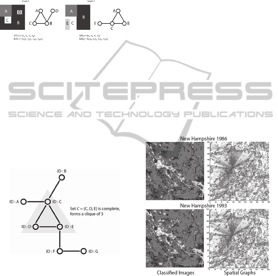
An example is shown in Figure 2. In this operation

the changes included the removal of node v

, edge

, and the addition of node v

, edge v

. If the cost

of each edit operation is equal to 1, then the total edit

distance d(G1, G2) is 4.

Figure 2: Conceptual example of GED.

GED serves as the most basic analysis of graph-

based landscapes. After this, extraction of subgraphs

in the form of cliques, communities and equivalences

will be initiated.

4.3 Landscape Cliques

The term clique as used in graph theory was coined

by Luce and Perry (1949). Similar to its usage in the

social context, cliques of graphs define tightly

connected set of nodes. A clique from an undirected

graph G = (V, E) is a subgraph of G with vertex set C

∈ V, in which every pair of nodes in C is connected

to every other by an edge (see Figure 3). In other

words, a clique is a complete subgraph of a graph.

Figure 3: Conceptual example of GED.

Landscape ecology discusses the formation of

landscape components from agglomeration of smaller

landscape elements (Wiens, 2002). Cliques can be

seen as landscape components, where tightly

arranged landscape elements are relationally

interdependent on each other. The existence of a

clique demonstrates that certain compatibility

characteristics exist between landscape elements,

while its persistence through time suggests the

importance of juxtaposition between those landscape

elements in supporting their resilience. Therefore

identifying types of cliques in a landscape graph and

monitoring their persistence through time may yield

fruitful insights on landscape structure.

5 DATA

In this phase of research, we use two classified

temporal land-cover datasets from Great Bay, New

Hampshire were used for demonstration purposes.

Pre-classified images were acquired from the Coastal

Change Analysis Program. The NOAA C-CAP

project used Landsat Thematic Mapper imagery for

land-cover classification at the full 30m pixel

resolution. Our analysis is based on the patchy

landscape mosaics built from these classes. The time

span for the Great Bay data set is 7 years (1986 to

1993). For the purpose of clarity, the demonstration

area is restricted to a 5 x 5 km region extracted from

the imagery (Figure 4).

In the final part of the research, time series sets of

Landsat images will be acquired, classified and be

implemented in STRG.

Figure 4: Demonstration study area.

6 EXPECTED OUTCOME

Currently GED had yielded us with satisfactory

results regarding the changing spatial relationships

between compatible/incompatible land types in our

SpatialTemporalRelationalGraphsonConnectedLandscapes

study area. Partially proving that the configuration of

landscape elements is not a random act of placement,

but is driven by compatibility and processes between

different landscape elements. To further our

understanding on configurations of landscape

elements, we are exploring the existence and meaning

of subgraphs in the form of landscape cliques. The

existence of assemblages such as cliques is strong

indications that complex landscape configurations

can also be formed. It is expected this kind of

topological subgraph extraction will provide even

better evidence on the existence of landscape

patterns. The result from subgraph analysis will be

used to empirically support the concept of connected

landscapes. In total, four published research papers

are expected at the end of this study. The first paper

focuses on construction of STRG, the second paper

focuses on extraction of subgraphs from STRG, the

third focuses on analytical methods of subgraph

patterns, and finally the fourth paper is a case study

paper combining the effort of STRG with that of

traditional spatial statistics.

7 STAGE OF RESEARCH

From our current results, we are confident that a

framework based on STRG can provide a sound

foundation for empirically supporting concepts from

landscape connectivity and interacting landscape

elements.

As mentioned, the entire research is comprised of

four components, which translates to four research

papers. The STRG as a data structure is fully

developed and the International Journal of GIS has

accepted a paper regarding this aspect. The usage of

GED as a form of relational change detection has also

been fully documented and ready to be submitted. At

the moment we are exploring how subgraphs can be

extracted from the data structure, and also their

semantic meanings after they are extracted. At the

same time, we are consulting with domain experts

(landscape ecologists) regarding possible meanings

with the extracted subgraphs. The remainder of the

research including writing up of papers is expected to

take one year.

REFERENCES

Gaucherel, C., et al., 2012. Understanding patchy landscape

dynamics: towards a landscape language. PLoS ONE,

7(9).

Kupfer, J. A., 2012. Landscape ecology and biogeography:

rethinking landscape metrics in a post-FRAGSTATS

landscape. Progress in Physical Geography, 36: 400-

420.

Luce, R. D. and Perry, A. D. 1949. A method of matrix

analysis of group structure. Psychometrika, 14(1), 95 -

116.

Pascual-Hortal, L. and Saura, S., 2006. Comparison and

development of new graph-based landscape

connectivity indices: towards the priorization of habitat

patches and corridors for conservation. Landscape

Ecology, 21: 959-967.

Takeyama, M. and Couclelis, H., 1997. Map dynamics:

integrating cellular automata and GIS through Geo-

Algebra. International Journal of Geographical

Information Science, 11: 73–91.

Thibaud, R., et al., 2013. A spatio-temporal graph model

for marine dune dynamics analysis and representation.

Transactions in GIS, 17: 742-762.

Troll, C., 1939. Luftbildplan und ökologische

Bodenforschung. Ihr zweckmäßiger Einsatz für die

wissenschaftliche Erforschung und praktische

Erschließung wenig bekannter Länder. In: KAYSER,

K. ed. Zeitschrift der Gesellschaft für Erdkunde zu

Berlin. Berlin.

Wiens, J. A. 2002. Riverine landscapes: taking landscape

ecology into the water. Freshwater Biology, 47, 501-

515.

GISTAM2015-DoctoralConsortium